NCAP City Air Quality Analysis: Baselines, Targets and Honest Progress Tracking

India's National Clean Air Programme set a national target for reducing particulate pollution across more than 130 non-attainment cities, and in doing so created a measurement problem as large as the pollution problem. Cities must demonstrate progress against a baseline year, using monitoring networks that have expanded substantially since that baseline was set, in a climate where year-to-year weather variability moves annual means by more than most control programmes achieve. Analysing NCAP progress honestly is genuinely difficult, and the difficulty is almost entirely analytical rather than political.

This guide covers the analysis: how baselines are constructed and where they go wrong, what the target actually means, how to separate real progress from network and weather artefacts, how source apportionment shapes the action plan, and how to build a city air quality report that stands up.

NCAP city air quality analysis is the assessment of progress against India's National Clean Air Programme targets for non-attainment cities, requiring construction of a defensible baseline, tracking of annual particulate concentrations against that baseline, correction for monitoring network changes and meteorological variability, source apportionment to direct the city action plan, and evaluation of implemented measures against measured outcomes.

What NCAP Requires

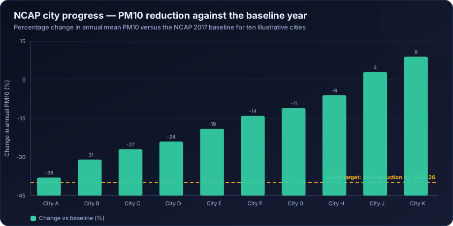
The programme identified cities that consistently failed to meet NAAQS over a multi-year assessment period — the non-attainment cities — and required each to prepare and implement a city-specific action plan, with a national target for reduction in particulate concentrations against a 2017 baseline. The target was subsequently revised and the timeline extended, and performance is tracked through the PRANA portal.

Each city action plan covers a standard set of sectors:

Sector	Typical measures
Road dust	Mechanical sweeping, water sprinkling, paving, greening of verges
Vehicles	Fleet modernisation, PUC enforcement, public transport, electrification
Industry	Fuel switching, control equipment, relocation, CEMS
Construction and demolition	Dust screens, covered transport, C&D waste processing
Biomass and waste burning	Enforcement, alternative disposal, community awareness
Domestic fuel	LPG access, clean cookstoves
Monitoring	Network expansion, CAAQMS installation, source apportionment studies
Public awareness	AQI dissemination, health advisories

The analytical work sits underneath all of it: which sectors matter most in this city, what the baseline actually was, and whether the measures are working.

Building a Defensible Baseline

The baseline determines everything, and it is where most NCAP analyses are weakest.

Problems with the 2017 baseline

Sparse monitoring. Many non-attainment cities had one or two manual monitoring stations in 2017. An annual mean from a single manual station sampling twice weekly carries wide uncertainty, and it certainly does not characterise a city.

Manual sampling limitations. Twice-weekly 24-hour samples give roughly 104 measurements a year. That is the NAAQS minimum, and it is thin for a baseline against which a decade of policy will be judged. Sampling day selection biases the result if it is not genuinely uniform.

PM10 versus PM2.5. The baseline and target are framed in PM10, largely because that is what most cities measured in 2017. PM2.5 has the stronger health basis, and a city can reduce PM10 substantially through dust control while PM2.5 barely moves — a genuine improvement in one metric and not in the one that matters most for health.

Meteorological anomaly. If 2017 happened to be a meteorologically unfavourable year in a given city, the baseline is inflated and the target correspondingly easier. If favourable, the reverse. Nobody chose the baseline year for its meteorology.

Constructing a better baseline

• Use multiple years where data exists — a three-year average centred on the baseline year is far more stable than a single year.
• Restrict to consistently operating stations. The baseline must be computed from the same stations used for subsequent comparison, or the comparison is invalid.
• State data capture for the baseline year explicitly.
• Meteorologically normalise the baseline using the same method applied to later years, so like is compared with like. See meteorological normalisation.
• Report the uncertainty on the baseline figure. A baseline of "138 ± 19 µg/m³" changes how a 15% reduction should be interpreted.

The Network Expansion Problem

This is the single largest artefact in NCAP progress tracking, and it works in both directions.

Cities have added stations since 2017, often substantially, as the network expansion recorded on the CPCB PRANA portal shows. If the new stations are in cleaner residential or peripheral areas, the city average falls without any emission change. If they are sited at hotspots — as they often are, since hotspots are where cities want to measure — the average rises.

The correction is straightforward and frequently omitted: compute the trend using only stations with continuous records across the full period. Report that consistent-station trend as the headline, and present the all-station average separately as a description of current status. Mixing the two produces a number that means nothing.

Other network artefacts to check:

• Method changes — a manual gravimetric station replaced by a BAM can introduce a systematic step
• Station relocations, even short distances
• Changes in validation practice as networks professionalised
• Changes in data capture, particularly if early years captured mostly one season

The check is to plot station metadata alongside the trend and annotate every change. If a step in the city average coincides with a network change, that is the explanation until proven otherwise.

Meteorological Normalisation for City Trends

Year-to-year meteorological variability in Indian cities routinely moves annual mean PM10 by 15–30%. NCAP targets are of a similar magnitude. Without normalisation, a city cannot distinguish policy success from a favourable monsoon.

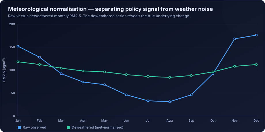
The honest presentation for a city report is a decomposition:

Observed annual mean PM10 fell from 138 µg/m³ (2017) to 104 µg/m³ (2024), a reduction of 24.6%. Meteorological normalisation attributes approximately 8 percentage points of this to more favourable meteorology in the later period, leaving an emissions-driven reduction of approximately 17%. The consistent-station subset (7 of 14 stations) shows a comparable normalised reduction of 16%.

That paragraph is defensible. "PM10 down 24.6%" is not, because it will not survive the first competent question.

Source Apportionment: What Actually Drives the Action Plan

An action plan built without source apportionment allocates effort by assumption. Nearly every Indian city that has conducted a proper study has found at least one surprise — biomass burning larger than expected, secondary aerosol dominating, or road dust smaller than the sweeping budget implied.

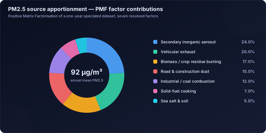
Three findings recur and each has direct planning implications:

Secondary inorganic aerosol is often the largest single factor. It is not a local source — it forms from SO2, NOx and NH3 emitted potentially hundreds of kilometres away. A city cannot control it within its boundary, which means an airshed-level strategy is required and the city's own action plan has a ceiling on what it can achieve.

Road dust is usually smaller in PM2.5 than in PM10. Dust control programmes deliver visible PM10 reductions and much less PM2.5 benefit. Since PM2.5 carries the health burden, a plan judged on PM10 can succeed on its metric while under-delivering on health.

Biomass and waste burning is frequently underestimated in inventories and prominent in receptor model results, particularly in winter.

The methods are covered in source apportionment of particulate matter, and the emission inventory side in emission inventory for dispersion modelling.

Evaluating Whether Measures Worked

Attributing a change to a specific intervention requires more than before-and-after comparison.

Interrupted time series. Model level and trend before the intervention, test whether either changed at the known implementation date, controlling for seasonality and meteorology. Far stronger than comparing two annual means.

Control comparison. A comparable city or a part of the same city that did not receive the intervention. Difference-in-differences between treated and control removes shared regional trends and weather.

Dose-response within the city. If mechanical sweeping was deployed in some wards and not others, compare them. Spatial heterogeneity in implementation is an analytical asset.

Bottom-up cross-check. Estimate the emission reduction the measure should have produced from activity data, convert it to an expected concentration change via dispersion modelling, and compare against what was observed. Large discrepancies indicate either implementation shortfall or a measurement problem, and both are worth knowing.

Placebo testing. Apply the analysis at a rural background station. If the "intervention effect" appears there too, it was regional, not local.

A Complete City Air Quality Analysis Programme

1. Network assessment — how many stations, sited where, in what land-use classes, with what capture rate, and are they adequate to characterise the city? Most non-attainment cities remain under-monitored relative to their area and population.
2. Data validation — full QA/QC on the historical record, which frequently changes the baseline itself.
3. Baseline reconstruction — multi-year, consistent-station, meteorologically normalised, with stated uncertainty.
4. Trend analysis — seasonal Mann-Kendall and Theil-Sen on the consistent-station series, per trend analysis methods.
5. Spatial analysis — interpolated and population-weighted exposure surfaces, hotspot identification, per GIS mapping.
6. Emission inventory — gridded, sector-resolved, at a resolution useful for planning.
7. Source apportionment — receptor modelling cross-checked against the inventory.
8. Dispersion modelling — scenario testing of proposed measures before they are funded.
9. Health burden assessment — exposure-based, so measures can be ranked by health benefit rather than by concentration reduction alone. See health risk assessment.
10. Progress reporting — honest, normalised, with uncertainty and artefacts disclosed.

What Honest Progress Reporting Looks Like

• Consistent-station trend as the headline metric, all-station status reported separately
• Meteorologically normalised alongside raw values, with the decomposition stated
• Both PM10 and PM2.5, since the target metric and the health metric differ
• Data capture and network changes disclosed, with change dates annotated on charts
• Uncertainty on every headline number
• Measure-level evaluation where the design allows, and an explicit statement where it does not
• Population-weighted exposure, not just station averages
• Clear separation of what the city controls from airshed-scale contributions it does not

Reports that do this are more useful and more credible than reports that produce a single confident percentage. They also survive scrutiny, which single confident percentages generally do not.

How DSTechnoverse Helps

DSTechnoverse supports urban local bodies, state pollution control boards, consultancies and research institutions working on city air quality programmes.

• Historical data validation and baseline reconstruction — full QA/QC on the archive, consistent-station baselines, multi-year averaging, meteorological normalisation and stated uncertainty.
• Network assessment and design — evaluation of whether the existing network can support the claims being made, and design of expansion including CAAQMS siting, manual stations and sensor networks for spatial density.
• Trend and progress analysis — seasonal Mann-Kendall and Theil-Sen on consistent-station series, network artefact review, and normalised versus raw decomposition.
• Source apportionment — study design, laboratory coordination, PMF execution and interpretation, cross-checked against the emission inventory.
• Emission inventory development — gridded, sector-resolved inventories at planning resolution.
• Scenario modelling — dispersion modelling of proposed measures so the action plan is prioritised by expected effect before budgets are committed. See our AERMOD service.
• Exposure and health burden — population-weighted exposure surfaces and attributable burden estimates, so measures can be ranked by health benefit.
• Progress reporting — city air quality reports written to withstand technical and public scrutiny, with artefacts, uncertainty and limitations disclosed.

The consistent principle is that a city is better served by a defensible 16% than an indefensible 25%, because the defensible number survives review and the indefensible one eventually costs credibility that is hard to recover.

---

Need air quality data turned into a defensible answer? DSTechnoverse provides end-to-end air quality analysis services — monitoring data validation, statistical analysis, source apportionment, dispersion modelling, GIS mapping, and regulator-ready reporting. Talk to our air quality team about your dataset or project.

Frequently Asked Questions

What is the National Clean Air Programme?

NCAP is India's national programme to reduce particulate air pollution in cities that consistently failed to meet ambient air quality standards. It designated more than 130 non-attainment cities, required each to prepare and implement a city-specific action plan, and set a national reduction target against a 2017 baseline, tracked through the CPCB PRANA portal.

How is NCAP progress measured?

Primarily by comparing annual mean PM10 concentrations against the city's baseline year. Defensible measurement also requires using only stations with continuous records across the period, correcting for meteorological variability, disclosing data capture, and reporting PM2.5 alongside PM10 since the health burden follows the finer fraction.

Why does network expansion complicate NCAP progress tracking?

Because cities have added monitoring stations since the baseline year, and new stations change the city average regardless of emissions. Stations added in cleaner areas lower the average; stations added at hotspots raise it. The correction is to compute the trend using only consistently operating stations and report the all-station average separately.

Why is meteorological normalisation important for city air quality targets?

Because year-to-year weather variation can change annual mean concentrations by 15–30% — comparable to or larger than the reduction targets themselves. Without normalisation, a city cannot demonstrate that an observed improvement came from its action plan rather than from a favourable monsoon or windier winter.

Why does the NCAP target use PM10 rather than PM2.5?

Largely because PM10 was what most cities measured in 2017, so it was the only parameter with a usable baseline. PM2.5 has the stronger health evidence base, and because dust control reduces PM10 far more than PM2.5, progress on the target metric can overstate progress on health. Reporting both is good practice.

What role does source apportionment play in a city action plan?

It determines which sectors actually dominate the burden, which sets realistic ceilings on what each intervention can achieve and prevents effort being allocated by assumption. Cities that have conducted proper studies frequently find that secondary aerosol or biomass burning is larger than expected and road dust smaller than the budget implied.

How can a city prove that a specific measure worked?

Through an interrupted time series analysis with a known implementation date, meteorological normalisation, and ideally a control comparison — a similar city or an unimplemented ward — plus a bottom-up cross-check estimating the expected emission reduction and modelling its concentration effect. Before-and-after comparison of annual means alone is not sufficient.

Can a city meet NCAP targets through its own actions alone?

Not always. Where source apportionment shows that secondary inorganic aerosol or regionally transported pollution dominates, a substantial share of the burden originates outside municipal boundaries and outside municipal control. Those cities need airshed-level coordination, and their action plans should state explicitly what fraction of the problem is locally addressable.