Source Apportionment of Particulate Matter: PMF, CMB and Finding Where Pollution Comes From

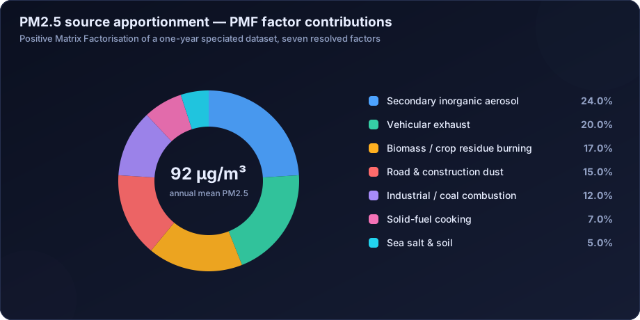
Knowing that PM2.5 is 92 µg/m³ tells you there is a problem. Knowing that 24% of it is secondary inorganic aerosol, 20% vehicular exhaust, 17% biomass burning and 15% road dust tells you what to do about it. That second statement is the product of source apportionment — the set of methods that decompose measured pollution into the sources responsible for it. It is the most policy-relevant output in air quality science, and also the most frequently misunderstood.

This guide covers source apportionment as practised: the chemical speciation that makes it possible, the marker species that identify each source, how Positive Matrix Factorisation and Chemical Mass Balance actually work, how factors are interpreted, where the uncertainty lies, and how the results should and should not be used.

Source apportionment is the analytical process of quantifying the contribution of different emission sources to measured ambient pollutant concentrations. Receptor models such as Positive Matrix Factorisation (PMF) and Chemical Mass Balance (CMB) work backwards from chemically speciated measurements at a receptor site to the source mix that produced them, complementing forward dispersion models that work from known emissions to predicted concentrations.

Two Directions of Attack: Receptor Models and Dispersion Models

There are two fundamentally different ways to link sources to concentrations, and mature studies use both.

	Receptor models (PMF, CMB, PCA)	Dispersion models (AERMOD, CALPUFF)
Direction	Measured concentrations → sources	Known emissions → predicted concentrations
Primary input	Speciated ambient measurements	Emission inventory, meteorology, terrain
Strength	Captures all real sources, including unknown and fugitive ones	Spatially resolved, predictive, scenario-capable
Weakness	Cannot predict future scenarios; needs long speciated datasets	Only as good as the inventory; misses unlisted sources
Best use	Diagnosing what is actually there now	Testing what a proposed change will do

Receptor models answer "what is in the air and where did it come from?" Dispersion models answer "what will happen if we build this or control that?" A city action plan needs both; an Environmental Clearance study typically needs the dispersion side, covered in our air dispersion modelling guide.

Where they disagree, that disagreement is a finding. If PMF says biomass burning is 17% and the emission inventory contains almost no biomass source, the inventory is incomplete. This cross-check has repeatedly revealed missing sources in Indian city inventories.

The Foundation: Chemical Speciation

Source apportionment is impossible from mass concentration alone, because a microgram of dust and a microgram of diesel soot are indistinguishable by weight. What distinguishes them is chemistry.

A speciation programme collects PM on filters and analyses them for:

Species group	Typical analytes	Analytical method
Carbonaceous	Elemental carbon (EC), organic carbon (OC)	Thermal-optical analysis
Water-soluble ions	SO4²⁻, NO3⁻, NH4⁺, Cl⁻, K⁺, Na⁺, Ca²⁺, Mg²⁺	Ion chromatography
Trace and crustal elements	Al, Si, Ca, Fe, Ti, Zn, Pb, Ni, V, As, Cu, Mn, Br	ICP-MS, XRF, or AAS
Organic markers	Levoglucosan, hopanes, steranes, PAHs	GC-MS

Sampling requirements are demanding. PMF needs a long dataset — 100 samples is a practical minimum, 150 or more is comfortable — with each sample speciated for 20 or more species and, critically, with uncertainty estimates and detection limits reported for every species. A speciation programme without documented uncertainties cannot be run through PMF properly, and retrofitting them afterwards is guesswork.

Marker Species: How Sources Reveal Themselves

Each source type leaves a distinctive chemical fingerprint. These are the associations that let an analyst interpret a mathematical factor as a physical source.

Source	Primary markers	Supporting evidence
Vehicular exhaust (diesel)	EC, high EC/OC ratio	Hopanes, steranes, Zn, Cu from lubricant and brake wear
Vehicular (petrol)	OC, CO co-variation	Lower EC/OC than diesel
Biomass / crop residue burning	K⁺, levoglucosan	High OC, Cl⁻, characteristic seasonality
Coal combustion	SO4²⁻, Se, As	Often with high SO2 co-variation
Crustal / road dust	Al, Si, Ca, Fe, Ti	Coarse-fraction dominance, low PM2.5/PM10 ratio
Secondary inorganic aerosol	SO4²⁻, NO3⁻, NH4⁺ together	Regional, low diurnal variability, weak wind-direction dependence
Sea salt	Na⁺, Cl⁻ in ratio ~0.55	Coastal sites, onshore wind sectors
Industrial / metallurgical	Source-specific metals — Pb, Ni, V, Cr, Mn	Sharp directional dependence
Solid-fuel cooking	OC, K⁺, indoor-outdoor gradient	Strong evening peak
Waste burning	Cl⁻, Sb, Cu, PAHs	Localised, episodic

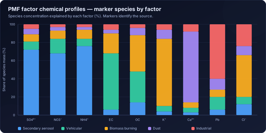
The chart above shows why the method works. Potassium loads almost entirely onto one factor; calcium onto another; sulphate, nitrate and ammonium together onto a third. Those loading patterns are the mathematical signature of biomass burning, dust and secondary aerosol respectively — and the interpretation is made by the analyst, not by the software.

Positive Matrix Factorisation (PMF)

PMF is the workhorse of modern source apportionment. The US EPA PMF model is freely available and is the de facto standard.

The model

PMF decomposes the measured data matrix X (samples × species) into two matrices:

X = G × F + E

• G = contributions matrix (samples × factors) — how much each factor contributed to each sample
• F = profiles matrix (factors × species) — the chemical fingerprint of each factor
• E = residuals

Two features distinguish PMF from ordinary factor analysis:

1. Non-negativity constraint. Both G and F are constrained to be non-negative, because a source cannot contribute negative mass. This alone makes the factors far more physically interpretable than PCA components.
2. Individual uncertainty weighting. Each data point is weighted by its own measurement uncertainty, so imprecise species near the detection limit do not dominate the fit. This is why species-level uncertainties are mandatory input, not optional.

The algorithm minimises the object function Q, the sum of squared uncertainty-scaled residuals.

Running a PMF study: the practical sequence

1. Assemble the data matrix — samples as rows, species as columns, with a parallel uncertainty matrix.
2. Categorise species as strong, weak or bad based on signal-to-noise ratio. Bad species are excluded; weak species are down-weighted, typically by tripling their uncertainty.
3. Handle values below detection limit — substitute half the detection limit with an inflated uncertainty, following the standard convention.
4. Choose the number of factors. This is the central judgement call. Run solutions from 3 to 10 factors and evaluate each on the Q/Qexpected ratio, the physical interpretability of the profiles, and the stability of the solution.
5. Assess rotational ambiguity using FPEAK, and apply constraints where a source profile is known.
6. Run error estimation — bootstrap (sampling uncertainty), displacement (rotational ambiguity), and bootstrap-displacement (both together). Any factor that is not stable across bootstrap runs should not be reported as a source.
7. Interpret the factors by comparing profiles against known source signatures.
8. Validate externally — check factor contributions against wind direction, season, known emission events, and the emission inventory.

Choosing the number of factors

This is where most PMF studies go wrong, in both directions:

• Too few factors merges distinct sources — diesel and petrol collapse into one "traffic" factor, or biomass and waste burning become one "combustion" factor. The result is under-informative but not wrong.
• Too many factors splits a single source across two, producing a "factor" with no physical meaning. Reporting it as a source is an error.

The diagnostics that help: a sharp drop in Q/Qexp when the correct factor count is reached; profiles that match known source signatures; contributions that vary sensibly with season and wind direction; and bootstrap stability above about 80% mapping.

Chemical Mass Balance (CMB)

CMB takes the opposite approach: instead of deriving profiles from the data, it requires them as input.

C_i = Σ (a_ij × S_j) — the measured concentration of species i is the sum across sources j of the source contribution S_j multiplied by the fraction a_ij of species i in source j's profile.

Given measured concentrations and a library of source profiles, CMB solves for the contributions by effective-variance least squares.

	PMF	CMB
Source profiles	Derived from the data	Must be supplied
Data required	Many samples (100+)	Can work on a single sample
Risk	Factor interpretation is subjective	Wrong or non-local profiles produce wrong answers
Handles unknown sources	Yes — they appear as factors	No — missing profile means missing source
Collinearity	Handled by the algorithm	Fails when two profiles are similar

CMB's dependence on local source profiles is its defining limitation in the Indian context. Profiles measured in the United States for gasoline vehicles do not describe an Indian two-wheeler fleet, an Indian brick kiln, or Indian crop residue. Studies that import foreign profiles without local measurement produce numbers that look authoritative and are not. Where local profiles exist, CMB is powerful, particularly for single-episode analysis where PMF's data requirement cannot be met.

Complementary Techniques

Receptor models are strongest when supported by simpler diagnostics:

• Bivariate polar plots — concentration plotted as a function of wind speed and direction simultaneously. A source at ground level appears as a hotspot at low wind speeds in one direction; an elevated stack appears at higher wind speeds.
• Conditional Probability Function (CPF) and Conditional Bivariate Probability Function (CBPF) — the probability that high concentrations come from a given direction.
• Potential Source Contribution Function (PSCF) — combines back trajectories with concentration data to identify regional source areas.
• Back-trajectory clustering using NOAA's HYSPLIT model to group airmass histories and compare concentrations between clusters.
• Ratio diagnostics — the PM2.5/PM10 ratio, EC/OC, toluene/benzene, and NOx/CO ratios each isolate specific source types cheaply.
• Enrichment factors — element concentration normalised to a crustal reference (usually Al or Ti) to separate natural from anthropogenic origin.

Interpreting the Results Correctly

Three interpretation errors recur:

Confusing a factor with a source. PMF produces mathematical factors. Calling one "vehicular exhaust" is an inference based on its chemical profile, its temporal pattern and its directional dependence. That inference should be stated as an inference, with its evidence.

Ignoring secondary aerosol attribution. Secondary inorganic aerosol is often the largest single factor, but it is not a source — it is a product. Its precursors (SO2, NOx, NH3) come from power plants, vehicles and agriculture, potentially hundreds of kilometres away. A control strategy that treats "secondary aerosol: 24%" as an unactionable category has missed the point; the actionable question is which precursor emissions to target.

Over-generalising in space and time. A receptor model describes the airshed at that receptor over that period. A one-year study at one urban station does not describe the whole city, and a winter campaign does not describe the year. Multi-site, multi-season designs cost more and are the only basis for a city-wide claim.

From Apportionment to Action

The value of source apportionment is that it ranks interventions by expected effect. If road dust is 15% and vehicle exhaust is 20%, then a road-sweeping programme has an addressable ceiling of 15% and a fleet-electrification programme a ceiling of 20% — before considering cost, feasibility or timescale.

The results feed directly into:

• City action plans under NCAP, where source shares determine sectoral targets
• Emission inventory validation, where mismatches reveal missing sources
• Dispersion modelling scenarios, where apportionment identifies which sources merit detailed modelling
• Health burden attribution, where source-specific exposure feeds health risk assessment
• Industrial fenceline disputes, where the question is whether a specific facility is responsible for a measured burden

How DSTechnoverse Helps

DSTechnoverse delivers source apportionment studies for cities, industrial clusters, individual facilities and research programmes.

• Study design — sampling site selection, seasonal coverage, sample count, species list and the uncertainty protocol, specified so the resulting dataset is actually usable in PMF rather than discovered to be unusable at the analysis stage.
• Laboratory coordination — specification and review of thermal-optical carbon analysis, ion chromatography and ICP-MS/XRF trace element work, including blanks, duplicates and detection limits.
• PMF execution — full EPA PMF workflow including species categorisation, factor number selection with documented diagnostics, FPEAK rotational analysis, and bootstrap, displacement and BS-DISP error estimation.
• CMB where appropriate — for episode analysis and where locally measured source profiles are available.
• Supporting diagnostics — bivariate polar plots, CPF/CBPF, HYSPLIT back-trajectory clustering, PSCF, and enrichment factor analysis.
• Interpretation and reporting — factors identified with their evidence, contributions quantified with uncertainty, and a control-strategy discussion that translates shares into ranked interventions.

We routinely cross-check apportionment results against the client's emission inventory and against dispersion modelling output, because agreement between an independent receptor model and a forward model is the strongest evidence an air quality study can present.

---

Need air quality data turned into a defensible answer? DSTechnoverse provides end-to-end air quality analysis services — monitoring data validation, statistical analysis, source apportionment, dispersion modelling, GIS mapping, and regulator-ready reporting. Talk to our air quality team about your dataset or project.

Frequently Asked Questions

What is source apportionment in air quality?

It is the analytical process of determining which emission sources are responsible for measured pollutant concentrations, and in what proportion. It converts a total concentration figure into a breakdown by source category — vehicles, industry, dust, biomass burning and so on — which is what makes targeted control strategies possible.

What is the difference between PMF and CMB?

PMF derives source profiles from the measured data itself and needs a long dataset of speciated samples. CMB requires source profiles to be supplied as input and can work on as few as one sample. PMF can reveal sources you did not know about; CMB can only apportion to the sources whose profiles you provide.

How many samples are needed for a PMF study?

At least 100 speciated samples is the practical minimum, with 150 or more preferred, each analysed for 20 or more species with documented uncertainties and detection limits. Fewer samples produce unstable factors that fail bootstrap testing and cannot be reported as sources with confidence.

What are marker species and why do they matter?

Marker species are chemicals strongly associated with a particular source — potassium and levoglucosan for biomass burning, elemental carbon for diesel exhaust, aluminium and silicon for crustal dust, sulphate and nitrate with ammonium for secondary aerosol. They are what allow an analyst to interpret a mathematical factor as a physical source.

Why is secondary aerosol often the largest contributor?

Because sulphate, nitrate and ammonium form in the atmosphere from precursor gases emitted by power plants, vehicles, industry and agriculture, and they accumulate over regional scales. It is a product rather than a source, so controlling it means controlling SO2, NOx and NH3 emissions, which may originate far from the receptor.

Can source apportionment identify a specific factory?

Sometimes, if that facility emits a distinctive marker element and the receptor is close enough for directional analysis to isolate it. More often, receptor models identify source categories rather than individual facilities. Attributing a burden to one named facility usually requires combining receptor results with dispersion modelling and fenceline monitoring.

How is source apportionment used in policy?

It ranks the sectors contributing to pollution, which determines where control effort should go and sets a realistic ceiling on what each intervention can achieve. City action plans under NCAP, emission inventory validation, and sectoral target-setting all depend on apportionment results.

Do receptor models replace dispersion modelling?

No — they answer different questions. Receptor models diagnose what is currently in the air and where it came from, including sources absent from any inventory. Dispersion models predict what concentrations a known set of emissions will produce, including for scenarios that do not yet exist. Strong studies run both and compare.