Air Quality GIS Mapping: Spatial Interpolation, Kriging and Exposure Surfaces

A table of station concentrations answers "how bad is it there?" A map answers "how bad is it where I live, where the school is, where the new housing is planned?" That second question is what drives planning decisions, health assessments and public concern, and answering it means predicting concentrations at locations where nobody measured. Spatial interpolation is how that prediction is made — and it is a modelling exercise with real uncertainty, not a drawing exercise.

This guide covers air quality GIS work end to end: the interpolation methods and when each is appropriate, land-use regression, dispersion model integration, population weighting, validation, and the cartographic decisions that make a map honest or misleading.

Air quality GIS mapping is the spatial analysis and visualisation of pollutant concentrations, using interpolation methods such as inverse distance weighting and kriging, statistical approaches such as land-use regression, or physically based dispersion model output, to produce continuous concentration surfaces from point measurements. These surfaces are combined with population, land-use and receptor data to quantify exposure and support planning and health assessment.

The Fundamental Difficulty

Air quality varies spatially on scales from metres to hundreds of kilometres simultaneously, and different pollutants vary on different scales.

Pollutant	Spatial variability	Implication for mapping
PM2.5	Largely regional, with local increments	Interpolates reasonably between stations
PM10	More local — dust sources are near-field	Interpolation less reliable
NO2	Strongly local, steep gradients near roads	Interpolation between distant stations fails badly
SO2	Point-source dominated, plume structure	Interpolation inappropriate; needs dispersion modelling
O3	Regional, smoothly varying, often higher outside cities	Interpolates well
CO	Local, traffic-dominated	Interpolation unreliable

The practical consequence: the same interpolation method that produces a defensible PM2.5 surface produces a misleading NO2 surface. NO2 falls by half within 100–200 metres of a major road; interpolating between two stations 5 km apart cannot represent that at all. For NO2, land-use regression or dispersion modelling is necessary.

Interpolation Methods

Nearest neighbour / Thiessen polygons

Assigns each location the value of the closest monitor, producing polygonal zones. Simple and transparent, and it produces obviously artificial discontinuities at polygon boundaries. Useful for administrative allocation — assigning a station to a ward — and poor as a physical representation.

Inverse Distance Weighting (IDW)

Predicts each location as a weighted average of surrounding measurements, with weight declining as distance raised to a power p (usually 2).

Strengths: simple, fast, exact at data points, easy to explain.

Weaknesses: produces bullseye artefacts around stations; cannot predict outside the range of observed values; no uncertainty estimate; the power parameter is chosen arbitrarily; and it ignores everything about the landscape.

Adequate for quick visualisation and dense networks. Not adequate for exposure assessment feeding a health study.

Spline interpolation

Fits a smooth minimum-curvature surface through the points. Produces attractive maps and can overshoot substantially between sparse points, generating values that no measurement supports. Use with caution and always inspect the range of the output.

Kriging

Kriging is the geostatistically correct approach. It models the spatial autocorrelation structure of the data explicitly through a variogram — a plot of how variance between pairs of points increases with separation distance — then uses that structure to compute optimal weights.

The variogram has three parameters that are themselves informative:

• Nugget — variance at zero separation, representing measurement error and micro-scale variability
• Sill — the variance at which the variogram plateaus, representing total spatial variance
• Range — the distance at which the plateau is reached; beyond this, locations are effectively uncorrelated

The range is the single most useful number in air quality spatial analysis. If the fitted range for PM2.5 is 25 km, then stations more than 25 km apart provide essentially no information about each other, and interpolation across a larger gap is extrapolation dressed as interpolation. Computing the variogram before mapping tells you immediately whether the network can support a map at all.

Kriging variants:

Variant	Use
Ordinary kriging	Unknown constant mean; the standard workhorse
Simple kriging	Known mean; rarely appropriate
Universal kriging	Underlying spatial trend present (e.g. urban-rural gradient)
Co-kriging	Uses a correlated secondary variable such as satellite AOD or NO2 emissions density
Regression kriging	Regress on covariates, then krige the residuals — usually the best practical choice
Indicator kriging	Probability of exceeding a threshold rather than the concentration itself

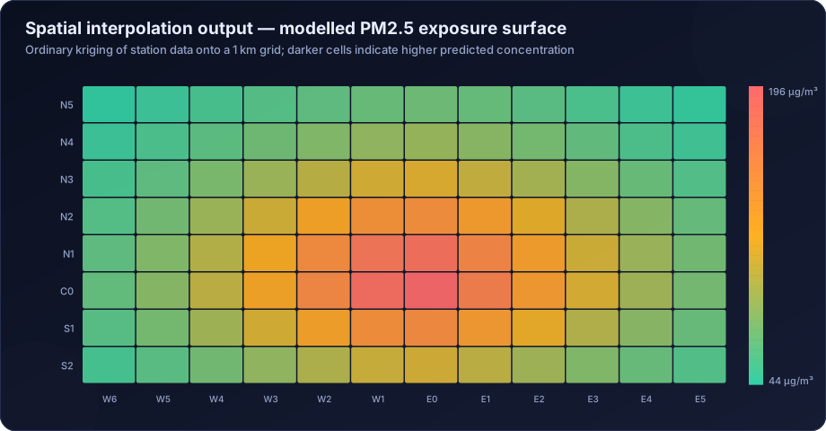
Kriging's decisive advantage is that it produces a prediction variance surface alongside the prediction. That map of uncertainty is arguably more important than the concentration map, because it shows exactly where the network is too sparse to support a claim — and it is almost never published.

Land-Use Regression (LUR)

Instead of interpolating between measurements, LUR builds a statistical model of concentration as a function of geographic predictors within buffers around each monitor:

• Traffic volume and road length within 50 m, 100 m, 300 m, 1,000 m buffers
• Land use — industrial, residential, commercial, green space areas
• Population and building density
• Elevation and distance to coast
• Distance to nearest major road, industrial estate, port

The fitted model is then applied to every grid cell. LUR handles the steep near-road gradients that interpolation cannot, and it is the standard method in urban epidemiological exposure assessment. It requires 20 or more monitoring sites for a stable model, which usually means a dedicated passive-sampler campaign rather than reliance on the regulatory network.

Dispersion model output

For point sources, a dispersion model produces a physically based concentration surface directly, accounting for stack parameters, plume rise, terrain and meteorology — see air dispersion modelling services and reading AERMOD contour maps. This is the correct approach for industrial impact assessment and the only one that supports scenario analysis.

Hybrid approaches

Best-in-class exposure surfaces combine everything: satellite AOD, dispersion model output, land-use predictors, meteorology and monitor data, fused in a machine-learning or Bayesian model. This is how modern national exposure products are built, and it is discussed further in satellite air quality data analysis.

Choosing a Method

Situation	Recommended approach
Dense network, regional pollutant (PM2.5, O3)	Ordinary or regression kriging
Sparse network	Do not interpolate; use LUR, dispersion or satellite-based methods
Near-road NO2 exposure	Land-use regression or dispersion modelling
Single industrial source	Dispersion modelling
Multiple industrial sources plus urban background	Dispersion modelling superimposed on an interpolated background
Regional to national scale	Satellite-based hybrid model
Quick visualisation for a presentation	IDW, clearly labelled as indicative

Validation

A concentration surface is a model prediction and must be validated as one.

Leave-one-out cross-validation (LOOCV) removes each monitor in turn, predicts its location from the remainder, and compares. Report R², RMSE, mean bias and the mean standardised error. This is the minimum.

Independent validation against monitors excluded entirely from model building is stronger, and essential for LUR and machine-learning surfaces, which will otherwise report performance that reflects memorisation.

Spatial validation matters more than aggregate metrics. Check whether errors cluster — if all the large residuals are in one part of the domain, the model is failing there specifically, and an overall R² will hide it.

Report the uncertainty surface. Kriging gives it directly; for other methods, bootstrap. A map without an uncertainty companion invites readers to trust the smooth parts of the surface as much as the well-measured parts.

Population Weighting and Exposure

A concentration surface becomes an exposure assessment when combined with population.

Population-weighted mean concentration = Σ (population in cell × concentration in cell) / Σ (population in cell)

Gridded population data — WorldPop, GHS-POP, or census data disaggregated to buildings — is overlaid on the concentration surface. The difference between the simple spatial mean and the population-weighted mean is often large, because people cluster in the more polluted urban core.

Further exposure metrics:

• Population exposed above a threshold — how many people live where the annual mean exceeds NAAQS or the WHO guideline
• Exposure distribution — the full histogram of population by concentration band, which is far more informative than a single mean
• Sensitive receptor exposure — concentrations at schools, hospitals, old-age homes, identified individually rather than averaged
• Equity analysis — exposure disaggregated by income, caste or settlement type, which frequently reveals that burden is not distributed evenly

These feed directly into health risk assessment.

Cartography: How Maps Mislead

Map design decisions change the conclusion a reader draws, and several common choices are actively misleading.

Classification scheme. Equal-interval, quantile, natural-breaks and standard-deviation classification of the same data produce visually different maps. Quantile classification always fills every class regardless of the data, so a clean city and a polluted one look equally variegated. For regulatory maps, use the standard's own breakpoints — the NAAQS limit, or the AQI category boundaries — so the classes mean something external.

Colour scheme. Use a sequential scheme for concentration and a diverging scheme only where there is a meaningful midpoint such as a standard. Avoid rainbow palettes: they create perceptual boundaries that do not exist in the data and are unreadable for colour-blind viewers.

Interpolating beyond the data. A smooth surface extending across a region with one monitor implies knowledge that does not exist. Either mask areas beyond the variogram range or overlay the uncertainty surface.

Omitting monitor locations. Always plot the stations. A reader must be able to see that the smooth green area in the north-west contains no measurements at all.

Scale and resolution mismatch. Presenting a surface interpolated from 8 stations at 100 m resolution implies spatial detail that the data cannot support. Match the output resolution to the information content.

Tools

Tool	Role
QGIS	Free, full-featured GIS; interpolation, mapping, spatial analysis
ArcGIS Pro	Commercial standard; Geostatistical Analyst for kriging
R (gstat, sf, terra, automap)	Scriptable geostatistics; the best environment for reproducible kriging
Python (geopandas, pykrige, rasterio, scikit-learn)	Scriptable spatial analysis and ML-based surfaces
SAGA GIS / GRASS GIS	Free, strong interpolation and terrain toolsets
Google Earth Engine	Satellite-scale processing without local downloads

For reproducibility, scripted approaches in R or Python are strongly preferable to desktop GIS click-workflows, for the same reasons set out in statistical analysis of air quality data in R and Python.

How DSTechnoverse Helps

DSTechnoverse produces air quality spatial analysis and mapping for city programmes, industrial projects, EIA studies and health assessments.

• Method selection — variogram analysis first, to establish whether the network can support interpolation at all, followed by the appropriate method: kriging, regression kriging, land-use regression, dispersion modelling or a hybrid.
• Surface generation — concentration surfaces at a resolution matched to the information content of the data, with the accompanying uncertainty surface always produced.
• Validation — leave-one-out and independent-station cross-validation, spatial residual analysis, and reported performance metrics rather than an unvalidated picture.
• Exposure analysis — population-weighted means, population above threshold, exposure distributions, sensitive receptor identification and equity analysis, using gridded population data.
• Dispersion integration — modelled industrial contributions superimposed on interpolated background, so incremental and cumulative impact are mapped consistently. See our AERMOD service.
• Cartography — maps classified against regulatory breakpoints, with perceptually uniform colour schemes, monitor locations shown, and areas beyond the data honestly masked.

Every surface we deliver comes with its validation statistics and its uncertainty map, because a concentration surface presented without them is a picture rather than a result.

---

Need air quality data turned into a defensible answer? DSTechnoverse provides end-to-end air quality analysis services — monitoring data validation, statistical analysis, source apportionment, dispersion modelling, GIS mapping, and regulator-ready reporting. Talk to our air quality team about your dataset or project.

Frequently Asked Questions

What is the best interpolation method for air quality data?

Kriging, and specifically regression kriging where covariates are available, because it models spatial autocorrelation explicitly and produces an uncertainty surface alongside the prediction. Inverse distance weighting is acceptable for quick visualisation with dense networks. For pollutants with steep local gradients such as NO2, interpolation is not appropriate at all and land-use regression or dispersion modelling should be used.

What is a variogram and why does it matter?

A variogram describes how the variance between measurement pairs increases with the distance separating them. Its range parameter — the distance beyond which locations are effectively uncorrelated — tells you directly whether your monitoring network is dense enough to support interpolation. If stations are further apart than the range, mapping between them is extrapolation.

Can I map air quality from just a few monitoring stations?

Generally not with interpolation. With fewer than about eight to ten stations, or with stations spaced beyond the variogram range, an interpolated surface implies spatial knowledge the data does not contain. Land-use regression, dispersion modelling or satellite-based estimation are more defensible in sparse-network situations.

What is land-use regression?

A statistical method that models pollutant concentration as a function of geographic predictors — traffic volume, road length, land use, population density, elevation — measured within buffers around monitoring sites. The fitted model is then applied to every grid cell. It captures steep near-road gradients that interpolation cannot and is standard in urban exposure epidemiology.

What is population-weighted exposure and why use it?

It is the mean concentration weighted by the number of people at each location, rather than a simple spatial average. It matters because population clusters in the more polluted urban core, so the simple spatial mean typically understates what people actually breathe — sometimes substantially.

Should an air quality map show uncertainty?

Yes, always. Kriging produces a prediction variance surface directly, and other methods can be bootstrapped. Without it, a reader has no way to distinguish a well-constrained area near several monitors from a smooth extrapolation across a region with none, and will trust both equally.

Which classification scheme should be used for air quality maps?

Wherever possible, the applicable standard's own breakpoints — the NAAQS limit or the AQI category boundaries — so class boundaries carry external meaning. Quantile classification is actively misleading for regulatory maps because it fills every class regardless of whether the data warrants it.

Which software is best for air quality GIS work?

QGIS is capable and free for general mapping and interpolation. R with gstat and sf, or Python with geopandas and pykrige, are better for reproducible geostatistics because the whole workflow is scripted. ArcGIS Pro's Geostatistical Analyst remains strong for interactive variogram fitting and kriging.