Meteorological Normalisation of Air Quality Data: Separating Policy Signal from Weather Noise

A city implements a major control programme. Two years later, PM2.5 has fallen 22% and the programme is declared a success. Then someone points out that the second year had 18% more rainfall, a longer monsoon, and mean wind speeds a third higher than the first. How much of the 22% was policy and how much was weather? Without meteorological normalisation, the honest answer is: nobody knows.

This is not a minor caveat. In most Indian cities, year-to-year meteorological variability can move annual mean PM2.5 by 15–30% with no change in emissions whatsoever. That is larger than the effect of most realistic control programmes. Any claim about the effectiveness of an intervention that has not been weather-normalised is, at best, unproven.

Meteorological normalisation, also called deweathering, is a statistical technique that removes the influence of weather variability from air quality time series so that the remaining variation reflects changes in emissions. The dominant modern approach trains a machine-learning model to predict concentration from meteorological and temporal variables, then repeatedly predicts concentration using meteorology randomly resampled from the whole record, producing a series that shows what concentrations would have been under average weather conditions.

Why Weather Dominates Measured Concentration

Ambient concentration is, to a first approximation, emission divided by dilution. Emissions change slowly; dilution changes hourly. The meteorological variables that control dilution:

Variable	Mechanism	Typical effect
Wind speed	Horizontal dilution and ventilation	Concentration roughly inversely proportional to wind speed
Wind direction	Determines which sources are upwind	Can change concentration several-fold between sectors
Mixing height	Vertical dilution volume	Winter nocturnal inversions at 100–200 m versus summer afternoons at 2,000+ m
Atmospheric stability	Rate of vertical mixing	Stable conditions trap emissions near the surface
Temperature	Photochemistry, heating demand, plume rise	Drives ozone formation and secondary aerosol
Relative humidity	Hygroscopic growth, aqueous chemistry	Enhances secondary aerosol formation and measured mass
Precipitation	Wet deposition and washout	Rapid, large reductions in PM
Boundary-layer ventilation index	Wind speed × mixing height	Single best composite predictor of accumulation

In the Indo-Gangetic Plain, the winter combination of low wind speed, shallow nocturnal boundary layer and high stability can multiply concentrations by four to five times relative to a summer afternoon with identical emissions. That is the noise a trend claim has to see through.

What Normalisation Does and Does Not Do

It does:

• Estimate what concentration would have been under a fixed, representative meteorological climatology
• Make years, seasons and locations comparable on an emissions basis
• Allow intervention effects to be estimated with far less confounding
• Reveal underlying trends hidden by weather variability

It does not:

• Prove causation on its own
• Remove the effect of emissions changes driven by weather — for example, less biomass heating in a mild winter is an emissions change, and normalisation will not distinguish it from a dilution effect
• Fix bad data; normalisation applied to unvalidated measurements produces confidently wrong output
• Substitute for a control group where one is available

Method 1 — Multiple Linear Regression

The classical approach models concentration as a linear function of meteorological predictors:

C = β₀ + β₁·(wind speed) + β₂·(temperature) + β₃·(RH) + β₄·(mixing height) + seasonal terms + trend term

The trend coefficient is then interpreted as the weather-adjusted change.

Its virtue is transparency: every coefficient is interpretable and the model can be written down in a report. Its limitations are serious in this domain:

• Relationships are strongly non-linear. Concentration versus wind speed is roughly hyperbolic, not linear.
• Interactions matter. Wind direction only matters at moderate speeds; humidity effects depend on temperature.
• Residuals are autocorrelated and skewed, so inference is unreliable without correction.

Log-transforming the concentration and adding polynomial or spline terms improves matters considerably, and a well-specified generalised additive model (GAM) with smooth terms for each meteorological variable is a genuinely good middle ground — flexible, still interpretable, and statistically well-founded.

Method 2 — Random Forest Normalisation (the Current Standard)

The approach developed by Grange and Carslaw has become the default in the peer-reviewed literature and in openair-based practice. It works in three stages.

Stage 1 — Train a predictive model

Fit a random forest predicting concentration from:

Meteorological predictors: wind speed, wind direction (as sine and cosine components, or as a numeric with the forest handling circularity), temperature, relative humidity, atmospheric pressure, precipitation, and where available mixing height or ventilation index.

Temporal predictors: Unix time (the trend carrier), Julian day (seasonality), hour of day, and day of week.

The inclusion of Unix time is essential — it is what allows the model to represent the long-term trend that normalisation is meant to expose.

Stage 2 — Resample the meteorology

This is the conceptual core. For each observation in the record:

1. Keep the temporal predictors — the actual date and time — fixed.
2. Randomly draw meteorological values from anywhere in the entire record (typically from a window of a few weeks around the same time of year, to preserve physical plausibility).
3. Predict the concentration under that resampled weather.
4. Repeat several hundred times and average the predictions.

The result is the concentration that would have been observed at that moment under randomly selected, and therefore average, meteorological conditions. Weather variability has been averaged out; the temporal trend remains.

Stage 3 — Analyse the normalised series

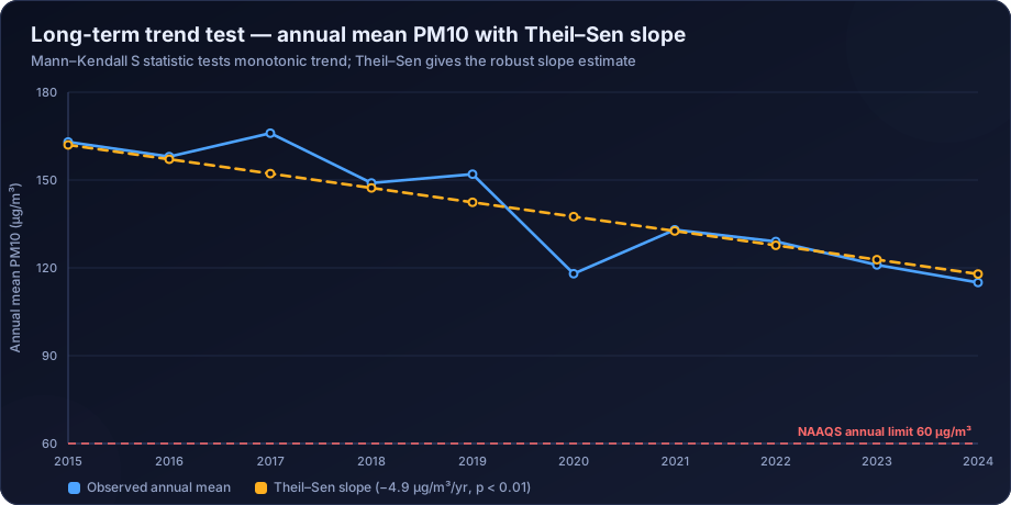
The deweathered series is then used for trend testing, intervention analysis and comparison across years or locations. Apply the same Mann-Kendall and Theil-Sen methods to the normalised series rather than the raw one.

Why random forests work well here

• They capture non-linearity and interactions automatically, without specification.
• They are robust to outliers and skewed distributions.
• They handle mixed variable types and missing values gracefully.
• Variable importance measures show which meteorological factors dominate, which is diagnostically useful in itself.

The trade-off is interpretability. A random forest is not a formula you can print, so the method section must describe the procedure and the validation rather than the model.

Method 3 — Gradient Boosting and Neural Networks

Gradient boosting machines (XGBoost, LightGBM) generally match or slightly exceed random forest accuracy on this task and train faster on large datasets. Neural networks can outperform both given very large datasets, at further cost in interpretability and tuning effort.

For most normalisation work the marginal accuracy gain over a random forest is small relative to the added complexity, and random forest remains the sensible default. The exception is when the normalisation model will also be used for forecasting, where boosting's edge is worth having — see air quality forecasting with machine learning.

Method 4 — Physical and Hybrid Approaches

Where a validated emission inventory exists, a chemical transport model can be run twice: once with actual meteorology and once with climatological meteorology, holding emissions constant. The difference isolates the meteorological effect physically rather than statistically.

This is the most rigorous approach and the most demanding — it requires a full CTM setup, a reliable inventory, and substantial computation. It is used in national policy evaluation and rarely in project-scale work. A practical hybrid is to use dispersion modelling output as an additional predictor in the statistical normalisation, which brings some physical structure into a tractable framework. Related predictive modelling is discussed in our air dispersion modelling guide.

Validation: How Do You Know the Normalisation Worked?

Normalisation is a model, and models must be validated.

1. Hold out time periods, not random rows. A random train-test split leaks information because adjacent hours are nearly identical. Hold out whole months or a whole year.
2. Report predictive performance on the held-out data — R², RMSE, mean bias — so the reader can judge how much of the variance the model actually explains. Typical values for a well-built PM2.5 model are R² of 0.6–0.8 on hourly data.
3. Check variable importance for plausibility. If day-of-week dominates wind speed, something is wrong.
4. Verify that normalised variance is much lower than raw variance. If it is not, the model has not captured the meteorological signal.
5. Test on a known event. A period with a documented emissions change — a lockdown, a plant shutdown, a fuel switch — should show up clearly in the normalised series.
6. Run a placebo test. Apply the method to a rural background station with no intervention. It should show no step change at the intervention date. If it does, the method is producing artefacts.

Interpreting Normalised Results

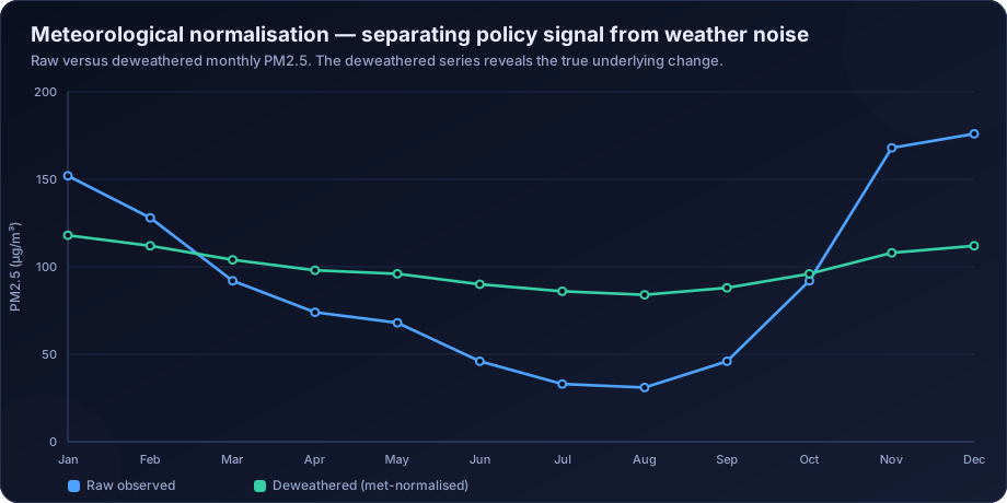
Reading the illustrative chart above: the raw series swings from about 30 to 175 µg/m³ across the year, dominated by seasonality and weather. The normalised series ranges from roughly 84 to 118 — the residual variation after weather is held constant. Two conclusions follow that the raw data could not support:

1. The seasonal amplitude is overwhelmingly meteorological. Emissions vary across the year, but far less than the raw curve suggests.
2. There is a modest underlying decline in the normalised series, which is the actual emissions signal.

A report using the raw data alone would attribute the seasonal swing to seasonal emissions and would miss or exaggerate the underlying trend. Both errors are common.

Reporting Normalised Results Honestly

• State the method, the predictor set, and the resampling scheme.
• Report model validation performance on held-out periods.
• Present raw and normalised series together, never normalised alone. Readers need to see what was removed.
• Quantify the meteorological contribution explicitly — "of the observed 22% decline, approximately 9 percentage points are attributable to more favourable meteorology and 13 to reduced emissions."
• State the limitations, particularly that weather-driven emission changes are not separated.
• Provide uncertainty. Bootstrap the whole procedure to produce a confidence band around the normalised series.

Where Normalisation Is Essential

• Policy and intervention evaluation — the primary use case, and the one where unnormalised claims are most often challenged.
• NCAP city progress reporting, where cities are compared against a baseline year that may have had unusual weather.
• Industrial compliance history, where a facility wants to demonstrate that reduced ambient concentrations reflect its control investment rather than a mild season.
• Cross-city and cross-station comparison, where different meteorological regimes make raw concentrations incomparable.
• Long-term trend analysis of any kind.
• Lockdown and event studies, where the whole literature was complicated by the fact that many lockdowns coincided with meteorologically favourable periods.

How DSTechnoverse Helps

DSTechnoverse performs meteorological normalisation as a standard component of trend and intervention analysis.

• Model development — random forest and gradient-boosted deweathering models built on validated concentration and meteorological data, with predictor sets chosen for the site and season structure rather than copied from a template.
• Meteorological data assembly — station data, India Meteorological Department records, and reanalysis products such as ECMWF ERA5 including boundary-layer height, quality-checked and gap-treated before use, as described in our meteorological data guide.
• Rigorous validation — time-based holdout, held-out-period performance metrics, variable importance review, and placebo testing at control locations.
• Attribution — quantified decomposition of an observed change into meteorological and emissions components, with bootstrap confidence intervals.
• Reporting — raw and normalised series presented together, method and validation documented, and limitations stated plainly so the conclusion is defensible under review.

We apply the same discipline to trend analysis and to intervention studies where a control location is available, because the strongest evidence combines normalisation with a comparison group.

---

Need air quality data turned into a defensible answer? DSTechnoverse provides end-to-end air quality analysis services — monitoring data validation, statistical analysis, source apportionment, dispersion modelling, GIS mapping, and regulator-ready reporting. Talk to our air quality team about your dataset or project.

Frequently Asked Questions

What is meteorological normalisation of air quality data?

It is a statistical technique that removes the influence of weather variability from a pollutant time series, so that the remaining variation reflects emissions rather than dilution. The standard modern method trains a machine-learning model on meteorological and temporal predictors, then predicts concentrations under repeatedly resampled weather to produce a weather-neutral series.

Why is deweathering necessary for evaluating air quality policy?

Because year-to-year meteorological variation can change annual mean concentrations by 15–30% with no change in emissions at all — often more than a control programme achieves. Without normalisation it is impossible to say whether an observed improvement came from the intervention or from a windier, wetter year.

How does random forest normalisation work?

A random forest is trained to predict concentration from meteorological variables plus temporal variables including a long-term time index. For each observation, the temporal variables are held fixed while meteorological values are randomly resampled from the record, and the prediction is averaged over hundreds of resamples. This averages out weather while preserving the trend.

What meteorological variables are needed?

At minimum wind speed, wind direction, temperature and relative humidity. Better models add atmospheric pressure, precipitation and boundary-layer or mixing height, which is often the single most powerful predictor because it controls the dilution volume directly.

How do you validate a normalisation model?

By holding out whole time periods rather than random rows, reporting predictive performance on that held-out data, checking that variable importance is physically plausible, confirming that normalised variance is much lower than raw variance, and running a placebo test at a control location where no intervention occurred.

Does normalisation prove that a policy worked?

No. It removes a major confounder and makes the emissions signal visible, which strengthens the evidence considerably, but causal attribution also needs a defined intervention date, an interrupted time series design, and ideally a comparison location that did not receive the intervention.

What are the limitations of meteorological normalisation?

It cannot separate weather-driven emission changes — less heating in a mild winter is a genuine emissions reduction that normalisation will attribute to emissions, which is correct but can be misread as a policy effect. It also depends entirely on the quality of the input data, and machine-learning models sacrifice interpretability for accuracy.

Can normalisation be applied to short datasets?

Poorly. The method needs enough data to characterise the relationship between weather and concentration across the full range of conditions, which in practice means at least two to three years of hourly data. Applied to a few months, it will extrapolate beyond its training range and produce unreliable results.