"Air quality has improved by 24% since 2019." It is the sentence every city, every industry and every regulator wants to publish, and it is the sentence most likely to be wrong. Concentrations fall for many reasons — a windier year, a longer monsoon, a pandemic, a change in the monitoring network, a relocated station, a new instrument — and only one of those reasons is the one the claim implies. Trend analysis is the statistical machinery that separates a real, sustained change in emissions from the noise of weather and measurement.
This guide covers the methods that actually hold up: why ordinary least squares fails on air quality data, how the Mann-Kendall test and Theil-Sen estimator work, how to handle seasonality and autocorrelation, how to detect change points, how many years you need, and how to report a trend so the claim survives review.
Air quality trend analysis is the statistical assessment of whether pollutant concentrations show a real monotonic change over time. Because air quality data is right-skewed, seasonal, autocorrelated and gap-ridden, the standard approach uses the non-parametric Mann-Kendall test for significance and the Theil-Sen estimator for slope magnitude, applied after meteorological normalisation so that weather variability is not mistaken for emission change.
Why Ordinary Regression Fails on Air Quality Data
Fitting a straight line by least squares and quoting the p-value is the default instinct, and it violates almost every assumption the method requires.
| OLS assumption | What air quality data does | Consequence |
|---|---|---|
| Normally distributed residuals | Strongly right-skewed, approximately log-normal | p-values unreliable |
| Constant variance (homoscedasticity) | Variance rises with concentration; winters are far more variable than monsoons | Standard errors wrong |
| Independent observations | Strong day-to-day and hour-to-hour autocorrelation | Effective sample size far smaller than n; p-values wildly optimistic |
| No influential outliers | Episode days are extreme and real | Slope dragged by a handful of days |
| Linear relationship | Trends are often stepwise, following interventions | Linear slope misdescribes the change |
The autocorrelation problem is the most damaging. If today's PM2.5 strongly predicts tomorrow's, then 3,650 daily values do not contain 3,650 independent pieces of information — perhaps a few hundred. An OLS p-value computed as though they were independent will declare significance that does not exist. This is the single most common statistical error in air quality reporting, and it is easy to avoid.
The Mann-Kendall Test
The Mann-Kendall test asks a deliberately narrow question: is there a monotonic trend — consistently up or consistently down — regardless of shape or distribution?
How it works
For a series of n observations, compare every value with every later value and score the comparison:
- +1 if the later value is greater
- −1 if the later value is smaller
- 0 if they are equal
Sum all comparisons to get the S statistic. A large positive S means later values are systematically higher (upward trend); a large negative S means a downward trend; S near zero means no monotonic trend.
Under the null hypothesis of no trend, S is approximately normally distributed with mean zero and a variance that depends on n and on the number of tied values. Standardising S gives a Z statistic, from which a p-value follows in the usual way.
Why it is the right tool
- Distribution-free. It uses only the ranks of comparisons, so skewness is irrelevant.
- Robust to outliers. An extreme episode day contributes exactly one comparison per pair, the same as an ordinary day.
- Tolerant of missing data. Pairs involving missing values are simply not counted.
- Handles values below detection limit, which can be treated as tied.
Interpreting the result
| Result | Interpretation |
|---|---|
| Z < −1.96, p < 0.05 | Statistically significant decreasing trend |
| Z > +1.96, p < 0.05 | Statistically significant increasing trend |
| −1.96 ≤ Z ≤ +1.96 | No significant monotonic trend detected |
The test tells you whether, not how much. For magnitude you need a slope estimator.
The Theil-Sen Slope Estimator
Theil-Sen computes the slope between every pair of points in the series and takes the median of all those pairwise slopes. It is implemented directly as the TheilSen() function in the openair R package, which is the reference implementation most air quality practitioners use.
Its properties make it the natural companion to Mann-Kendall:
- It has a breakdown point of about 29%, meaning up to roughly 29% of the data can be arbitrarily corrupted before the estimate is destroyed. OLS has a breakdown point of 0% — one extreme point can move it arbitrarily.
- It makes no distributional assumption.
- Its confidence interval derives from the same rank statistics as Mann-Kendall, so significance and magnitude come from one coherent framework.
Reported properly, a trend result looks like this:
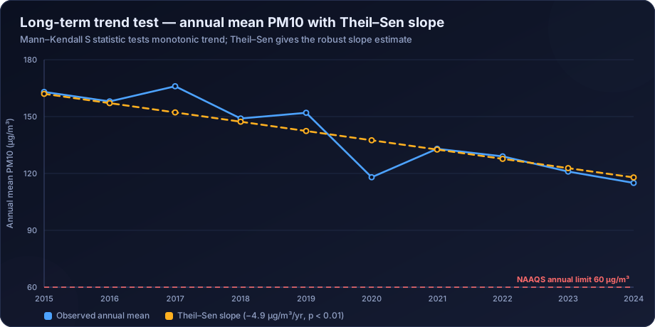
Annual mean PM10 at Station 3 declined by 4.9 µg/m³ per year (Theil-Sen slope; 95% CI −6.4 to −3.1), a statistically significant decreasing trend (Mann-Kendall Z = −3.14, p = 0.0017, n = 10 years, data capture ≥ 82% in all years).
Every element of that sentence is doing work. Magnitude, uncertainty, significance, sample size, and data quality. A trend claim missing any of them is incomplete.
Handling Seasonality: the Seasonal Mann-Kendall Test
Raw air quality data has an enormous seasonal cycle — winter concentrations can be five times monsoon concentrations. If a series starts in January and ends in July, the seasonal cycle alone will manufacture an apparent downward trend.
Two standard solutions:
Seasonal Mann-Kendall (Hirsch-Slack test). Compute the S statistic within each season separately — January values compared only with other January values, and so on — then sum the seasonal statistics and their variances. This compares like with like and removes seasonality entirely without any modelling assumption.
Deseasonalise first. Subtract a monthly climatology or fit and remove a seasonal component (STL decomposition is common), then run the standard test on the residual series.
For monthly data across several years, the seasonal Mann-Kendall test is the default and should be stated as such in the methods section.
Handling Autocorrelation
Even after deseasonalising, air quality series remain serially correlated: consecutive days share the same airmass and boundary-layer conditions. Positive autocorrelation inflates the apparent significance of any trend.
Three accepted corrections:
- Pre-whitening. Estimate the lag-1 autocorrelation coefficient and remove it from the series before testing. Simple, widely used, and known to reduce the power of the test somewhat.
- Trend-free pre-whitening (TFPW). Remove the Theil-Sen trend first, then pre-whiten the residuals, then add the trend back. This preserves power better than naive pre-whitening and is the recommended variant in most of the hydrology and air quality literature.
- Variance correction. Adjust the variance of S using an effective sample size derived from the autocorrelation structure, rather than modifying the data.
Whichever is applied, state it. A Mann-Kendall result with no mention of autocorrelation treatment invites the reviewer to assume none was applied.
Aggregation Level: What Should You Actually Test?
| Series tested | Advantages | Risks |
|---|---|---|
| Hourly | Maximum information | Extreme autocorrelation; seasonality; usually unnecessary |
| Daily (24-h averages) | Natural unit for PM standards | Strong autocorrelation and seasonality; use seasonal test |
| Monthly means | Manageable, standard for seasonal Mann-Kendall | Needs adequate within-month capture |
| Annual means | Removes seasonality entirely; the clearest headline | Only one point per year, so 10+ years needed for power |
| Annual percentiles (98th) | Tests the tail, which matters for compliance | Noisier than the mean |
A robust reporting practice is to run the test at two levels — monthly with a seasonal test, and annual on the means — and check they agree. Disagreement is itself informative: it usually indicates that the change is concentrated in one season.
How Many Years Do You Need?
Statistical power depends on the effect size relative to variability. Practical guidance:
- Fewer than 5 years: rarely enough to demonstrate anything but a very large change. Report descriptively, not as a trend.
- 5–8 years: capable of detecting large trends (roughly 5% per year or more) if variability is moderate.
- 10 years: the conventional minimum for a credible published trend statement.
- 15+ years: sufficient to detect modest trends and to identify change points reliably.
The reason is straightforward. A single anomalous year — an unusually strong monsoon, a lockdown, an exceptional stubble-burning season — can dominate a short series. In a 15-year series it is one point among many.
Change-Point Detection: When the Trend Is Not Monotonic
Air quality often does not change smoothly. It steps, when a fuel switch happens, a plant closes, a control device is commissioned, or a policy takes effect. Mann-Kendall on a stepped series returns a significant trend, but the linear slope misdescribes what happened.
Useful tools:
- Pettitt's test — non-parametric detection of a single change point in the mean, with a p-value.
- CUSUM (cumulative sum) charts — visual and quantitative detection of a shift in level.
- Bayesian change-point analysis — probabilistic identification of one or several change points with credible intervals.
- Piecewise (segmented) regression — once a change point is identified, fit separate slopes before and after.
Where an intervention date is known in advance, the honest analysis is an interrupted time series: model the level and slope before the intervention, and test whether either changed at the known date, controlling for seasonality and weather. That is a far stronger causal claim than a simple before-and-after comparison of means.
The Step Everyone Skips: Meteorological Normalisation
A trend test on raw data answers "did concentrations change?" It does not answer "did emissions change?" Those diverge whenever the weather in the later years differed from the earlier ones — which is always.
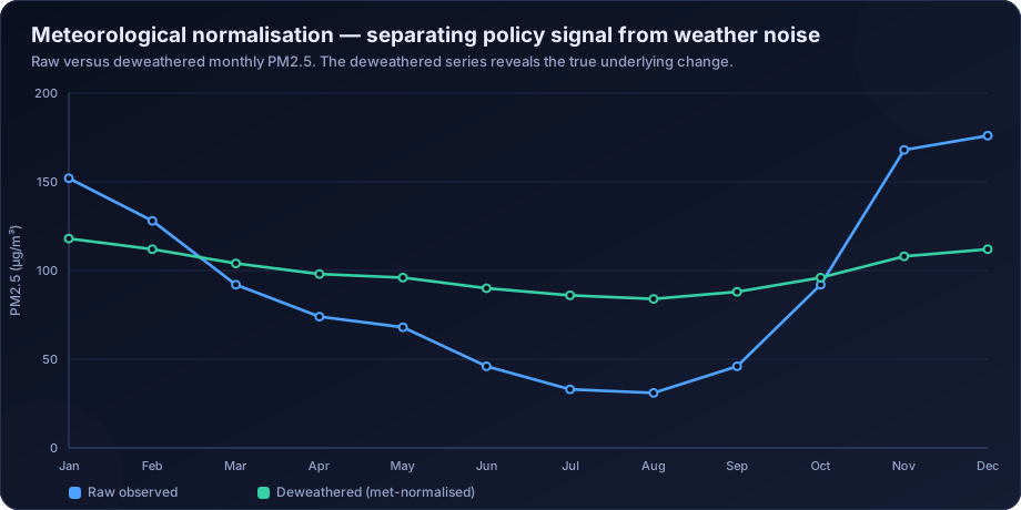
The chart shows the problem cleanly. The raw series has a massive seasonal swing that dominates any trend. The deweathered series — produced by modelling concentration as a function of meteorological variables and then predicting under a fixed, resampled climate — is much flatter and reveals the underlying change. In this illustrative case the raw data would support a dramatic-looking seasonal narrative while the normalised data shows a modest, steady underlying decline.
Full method treatment, including random-forest deweathering, is in meteorological normalisation of air quality data.
Network Artefacts That Masquerade as Trends
Before attributing a trend to emissions, rule out the mundane explanations:
- A station moved. Even 200 metres can change a kerbside station into a background station.
- An instrument was replaced. BAM to gravimetric, or one BAM model to another, can introduce a step of several µg/m³.
- Data capture changed. If early years captured mostly winter and later years captured evenly, the "improvement" is a sampling artefact.
- A validation policy changed. Tighter flagging in later years removes high artefacts and lowers the apparent mean.
- Stations were added to the network and the "city average" now includes cleaner suburbs.
- A nearby land-use change — a new flyover, a demolished factory, a construction site — altered what the station measures without any city-wide change.
The check is simple and rarely done: plot the metadata alongside the data. Station relocations, instrument changes and calibration events should appear as annotations on the trend chart.
Reporting a Trend Properly
A defensible trend statement contains:
- The parameter, station or aggregation, and period covered
- The averaging level tested (daily, monthly, annual)
- The test used, including the seasonal and autocorrelation treatment
- The Theil-Sen slope with confidence interval and units
- The Mann-Kendall Z and p-value
- Data capture per year
- Whether meteorological normalisation was applied and how
- Any network changes during the period
- A plain-language interpretation with appropriate caution
Anything less is a claim, not a result.
Worked Interpretation
Take the series in the chart above: annual mean PM10 falling from 163 to 115 µg/m³ over ten years.
- Naive statement: "PM10 fell 29%." True but uninformative — it compares two single years, either of which could be anomalous.
- Trend statement: Theil-Sen slope −4.9 µg/m³/yr, Mann-Kendall Z = −3.14, p = 0.0017. Significant and quantified.
- After normalisation: if the deweathered slope is −3.1 µg/m³/yr, roughly a third of the observed decline was favourable meteorology, and the emissions-driven improvement is real but smaller than the headline.
- With change-point analysis: if Pettitt identifies a break in 2020, the decline may be dominated by a single event rather than sustained progress, which changes the policy conclusion entirely.
All four statements come from the same data. Only the last two are useful.
How DSTechnoverse Helps
DSTechnoverse performs trend analysis for city air quality programmes, industrial compliance histories, NCAP progress reporting and research datasets across India.
- Method selection and execution — seasonal and standard Mann-Kendall, Theil-Sen slopes with confidence intervals, trend-free pre-whitening for autocorrelation, and change-point detection where the trend is not monotonic. All executed in R and Python so results are reproducible and auditable.
- Meteorological normalisation — random-forest deweathering and regression-based normalisation so that the reported trend reflects emissions rather than weather.
- Network artefact review — we reconstruct the station metadata history before analysing, because a relocation or instrument change explains more apparent trends than most people expect.
- Data preparation — validation, gap treatment and capture assessment first, as described in our QA/QC guide, because trend tests on unvalidated data amplify errors rather than reveal signal.
- Reporting — trend statements written with the full statistical apparatus, plus charts that show the data, the fitted slope, the confidence band and the annotated network events.
We also connect trend findings to forward-looking work: where a trend is deteriorating, dispersion modelling identifies which sources are driving it, and source apportionment quantifies the split.
Need air quality data turned into a defensible answer? DSTechnoverse provides end-to-end air quality analysis services — monitoring data validation, statistical analysis, source apportionment, dispersion modelling, GIS mapping, and regulator-ready reporting. Talk to our air quality team about your dataset or project.
Frequently Asked Questions
What is the Mann-Kendall test used for in air quality?
It tests whether a pollutant concentration series shows a statistically significant monotonic trend over time. Because it is non-parametric, it does not assume normally distributed data, is robust to extreme episode values, and tolerates missing observations — all of which make it far better suited to air quality data than ordinary least-squares regression.
What is the Theil-Sen slope and why use it?
The Theil-Sen estimator is the median of the slopes between all pairs of points in a series. It is highly resistant to outliers, with a breakdown point near 29% compared to zero for least-squares regression, and it makes no distributional assumption. It provides the magnitude of change that the Mann-Kendall test alone does not.
How many years of data are needed to establish an air quality trend?
Ten years is the conventional minimum for a credible published trend. Five to eight years can detect large changes if variability is moderate. Fewer than five years should generally be reported descriptively rather than as a trend, because a single anomalous year can dominate the result.
Why can't I just fit a straight line to the data?
Air quality data violates the assumptions behind ordinary least squares: the residuals are skewed rather than normal, the variance changes with concentration, and consecutive observations are strongly correlated. That last issue makes the effective sample size much smaller than the number of observations, so a naive p-value dramatically overstates significance.
What is seasonal Mann-Kendall and when is it needed?
The seasonal variant computes the trend statistic within each month or season separately and then combines them. It is needed whenever the data has a strong annual cycle — which is nearly always in air quality — because otherwise the seasonal pattern can create or mask an apparent trend depending on where the series starts and ends.
What is meteorological normalisation and why does it matter for trends?
It is the process of statistically removing the influence of weather so that the remaining variation reflects emissions. Without it, a windy, wet year looks like a policy success and a stagnant winter looks like a failure. Any trend claim intended to demonstrate the effect of an intervention needs normalisation to be credible.
How do you tell a real improvement from a monitoring artefact?
By reviewing the station metadata history alongside the data. Relocations, instrument replacements, changes in validation policy, changes in data capture, and additions to the network all produce apparent trends. These events should be annotated on the trend chart and explicitly ruled out before an emissions explanation is offered.
Can trend analysis prove that a control measure worked?
Not on its own. A trend test shows that concentrations changed; attributing that change to a specific intervention requires an interrupted time series design with a known intervention date, meteorological normalisation, and ideally a control location that did not receive the intervention. Without those elements the association remains circumstantial.