Low-Cost Air Quality Sensors: Calibration, Drift Correction and Data Quality

Low-cost air quality sensors have done something reference monitors never could: they have put air quality measurement in the hands of schools, resident associations, factory EHS teams and city departments, at a hundredth of the cost per node. They have also generated an enormous volume of data that is, in its raw form, wrong — often by 30 to 60% — in ways that are systematic, predictable and correctable. The difference between a useful sensor network and a misleading one is entirely a matter of calibration and data handling.

This guide covers what low-cost sensors actually measure, why raw output diverges from reference measurements, how to run a co-location campaign, which calibration models work, how to manage drift over a deployment's life, and where sensor data belongs in professional air quality analysis.

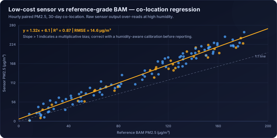
Low-cost air quality sensor calibration is the process of correcting raw sensor output against a reference-grade instrument through co-location, deriving a correction model that accounts for humidity, temperature and particle size effects, and maintaining that correction over time as the sensor drifts. Without calibration, optical PM sensors typically over-report concentrations substantially in humid conditions, and electrochemical gas sensors suffer cross-sensitivity and baseline drift that make raw readings unreliable.

What Low-Cost Sensors Actually Measure

Understanding the measurement principle explains every one of the failure modes.

Optical particulate sensors

A low-cost PM sensor is a nephelometer: it shines a laser through a small airstream and counts the light scattered by passing particles. From the scattering signal it estimates particle number by size bin, and from that it estimates mass concentration.

That last step is where the trouble starts. Converting scattered light into mass requires assumptions about:

• Particle density — soot, dust and sea salt have very different densities, and the sensor assumes one value.
• Refractive index — how strongly a particle scatters depends on its composition.
• Particle shape — the conversion assumes spheres; dust is not spherical.
• Size distribution — inferred from a small number of coarse bins.

The sensor is therefore measuring an optical property and reporting a mass. When the aerosol composition changes — winter combustion smoke versus summer dust — the assumed conversion no longer holds, and the error changes with it.

The humidity problem is the dominant one. Many atmospheric particles are hygroscopic: above roughly 70–75% relative humidity they absorb water and grow. A grown particle scatters far more light, so the sensor reports far more mass — but a reference gravimetric or BAM measurement, which conditions or heats the sample, does not see that water. This produces the classic pattern of severe over-reading on humid mornings and during monsoon, and it is the single largest correctable error in low-cost PM data.

Optical sensors also have a lower size cut around 0.3 µm, so they miss ultrafine particles entirely, and an upper limit around 10 µm with poor efficiency above 2.5 µm — which is why low-cost "PM10" readings are considerably less reliable than "PM2.5" readings.

Electrochemical gas sensors

Gas sensors for NO2, O3, CO and SO2 typically use electrochemical cells, where the target gas reacts at an electrode and produces a current proportional to concentration. Their characteristic problems:

• Cross-sensitivity. NO2 sensors respond to ozone; ozone sensors respond to NO2. Deployments frequently measure the sum and report it as one of them.
• Temperature dependence. Cell response varies substantially with temperature, requiring compensation.
• Baseline drift. The zero point moves over weeks to months.
• Limited lifetime. Electrolyte depletion typically limits useful life to one to two years.
• Poor low-concentration performance. At the low ambient concentrations typical for SO2 in India, the signal is often within the noise.

Metal-oxide (MOS) sensors are cheaper still and are generally unsuitable for quantitative ambient work — they respond to a broad class of reducing gases, drift substantially, and are strongly humidity-dependent.

The Co-Location Protocol

Calibration means comparing the sensor against a trusted reference under real conditions. This is not optional and it is not a one-off. The US EPA Air Sensor Toolbox publishes performance targets and testing protocols for exactly this purpose, and is the best available starting point.

Design requirements:

Element	Recommendation	Reason
Reference instrument	Reference or equivalent method (BAM, gravimetric, certified analyser)	The correction can only be as good as the reference
Duration	Minimum 2 weeks; 4–8 weeks strongly preferred	Must span a range of concentration and humidity
Seasonal coverage	Ideally one campaign per season	Aerosol composition changes; a monsoon calibration may not hold in winter
Placement	Inlets within 1–2 m, same height, same exposure	Otherwise you are calibrating against a spatial gradient
Time alignment	Synchronise clocks; average to a common interval	Misalignment destroys correlation
Concentration range	Must span the range the sensor will encounter	A calibration built at 20–60 µg/m³ will not extrapolate to 400
Replication	Co-locate several units of the same model	Reveals unit-to-unit variability

Unit-to-unit variability deserves emphasis. Two sensors of the same model, side by side, routinely differ by 10–20%. This means a single co-located unit cannot calibrate a whole fleet without an assumption of uniformity that is usually false. Either co-locate every unit before deployment, or characterise the fleet variability and report it as uncertainty.

Calibration Models

Once paired data exists, the correction model can range from trivial to sophisticated.

1. Simple linear regression

Reference = a + b × Sensor

Easy, transparent, and usually inadequate on its own because it cannot capture the humidity dependence. Useful as a baseline against which better models are judged.

2. Multiple linear regression with meteorological terms

Reference = a + b × Sensor + c × RH + d × T + e × (Sensor × RH)

The interaction term between sensor reading and relative humidity is what captures hygroscopic growth, and adding it typically produces the single largest improvement in fit. This model is interpretable, robust, and adequate for many deployments.

3. Humidity growth-factor correction

A physically motivated correction that divides the sensor reading by a hygroscopic growth factor derived from relative humidity — for example a Köhler-theory-based expression of the form 1 + κ·RH/(100−RH). Because it is physics-based rather than fitted, it often transfers better to new sites and seasons than a purely statistical model.

4. Machine learning models

Random forests and gradient boosting handle non-linear interactions between sensor output, humidity, temperature, time of day and season without the analyst specifying the functional form. They routinely outperform linear models on the co-location dataset.

The caution is real: they can overfit to the co-location conditions and degrade badly when applied outside the range or season in which they were trained. Any ML calibration must be validated on held-out data from a different period, not a random split of the same period.

Evaluating a calibration

Metric	What it tells you	Typical target for PM2.5
R²	Proportion of variance explained	> 0.80
RMSE	Typical error magnitude	< 25% of the mean
Mean bias	Systematic over- or under-reading	Near zero after correction
Slope	Multiplicative bias	Near 1.0
Intercept	Additive offset	Near 0
Error at high concentration	Performance where it matters most	Check separately

That last row matters more than the headline R². A calibration with excellent overall R² can still perform badly at the high concentrations that trigger health advisories, because those points are rare in the fitting dataset. Always evaluate error stratified by concentration band.

Managing Drift

Calibration is not permanent. Optical sensors accumulate dust on the optics and their laser output declines; electrochemical cells deplete. Both cause slow, systematic drift.

Drift management strategies:

• Periodic re-co-location — bring units back to the reference site every 3–6 months. Effective, and logistically demanding for a large network.
• A permanent reference anchor — keep one or more sensors permanently co-located with a reference instrument and use their drift as a proxy for the fleet.
• Network-based drift detection — compare each node against the network median. A node diverging steadily from its neighbours is drifting.
• Scheduled replacement — treat sensors as consumables with a defined service life rather than instruments to be maintained indefinitely.
• Continuous QA metrics — track each node's correlation with its neighbours, its noise level and its baseline; flag automatically when these degrade.

Any deployment without a drift-management plan will produce data whose quality degrades invisibly. The data keeps arriving and keeps looking plausible; it is simply increasingly wrong.

Where Sensors Are and Are Not Appropriate

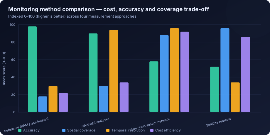
Appropriate uses:

• Spatial gradient mapping — resolving how concentration varies across a city, an industrial estate or a neighbourhood, at a density no reference network could afford.
• Hotspot identification — finding the locations that warrant a reference measurement.
• Fenceline and perimeter monitoring for industrial sites, where relative change and directional information matter more than absolute accuracy.
• Community engagement and education, where visible local data drives awareness.
• Real-time operational triggers — dust suppression on a construction site, ventilation control in a building.
• Filling temporal gaps in a sparse reference network.
• Indoor air quality, where reference-grade instruments are rarely deployed at all. See indoor air quality analysis.

Inappropriate uses:

• Regulatory compliance determination against NAAQS, which requires reference or equivalent methods.
• EIA baseline monitoring, where prescribed methods apply.
• Legal or enforcement evidence, where the measurement chain must be traceable and defensible.
• Long-term trend analysis across sensor generations, where drift and model changes create artefacts indistinguishable from real trends.
• Any published absolute concentration without a stated calibration and uncertainty.

Designing a Sensor Network

If sensors are the right tool, the design decisions that determine whether the network produces value:

1. State the question first. Gradient mapping, hotspot finding and operational triggering imply different node placements.
2. Anchor to reference. At least one node co-located with a reference monitor, permanently. A network with no anchor cannot be calibrated or drift-checked.
3. Co-locate the whole fleet before deployment, even briefly, to characterise unit-to-unit variability.
4. Design for maintenance — power, connectivity, physical access, and a replacement budget.
5. Log raw alongside corrected values. If the calibration model is later improved, raw data can be reprocessed; corrected-only data cannot.
6. Publish uncertainty with every value. A number without an uncertainty invites over-interpretation.
7. Plan the analysis pipeline — automated validation, drift flagging and correction applied continuously, not retrospectively.

How DSTechnoverse Helps

DSTechnoverse designs, calibrates and analyses low-cost sensor deployments for industrial fencelines, municipal programmes, campuses and research projects.

• Network design — objective definition, node siting, reference anchoring, and a maintenance and replacement plan sized to the deployment's life.
• Co-location campaigns — protocol design, execution against reference instruments, and full fleet characterisation including unit-to-unit variability.
• Calibration model development — from interpretable multiple regression with humidity interaction terms to gradient-boosted models, always validated on held-out periods rather than random splits, with performance reported by concentration band.
• Drift management — permanent reference anchoring, network-median divergence detection, automated QA metrics, and re-calibration scheduling.
• Data pipeline — automated ingestion, validation, correction and archiving, with raw values retained so data can be reprocessed when the calibration improves.
• Analysis and reporting — spatial mapping, gradient analysis, hotspot identification and integration with reference data, with uncertainty stated throughout.

Where sensor data indicates a problem that needs a defensible answer, we escalate to reference monitoring and dispersion modelling rather than over-claiming from the sensors — which is, ultimately, the discipline that makes sensor networks useful.

---

Need air quality data turned into a defensible answer? DSTechnoverse provides end-to-end air quality analysis services — monitoring data validation, statistical analysis, source apportionment, dispersion modelling, GIS mapping, and regulator-ready reporting. Talk to our air quality team about your dataset or project.

Frequently Asked Questions

Are low-cost air quality sensors accurate?

Not in raw form. Optical PM sensors typically over-report substantially at high humidity because hygroscopic particles grow and scatter more light, and electrochemical gas sensors suffer cross-sensitivity and baseline drift. After co-location against a reference instrument and application of a humidity-aware calibration, PM2.5 data can reach R² above 0.8 and become genuinely useful for relative and spatial analysis.

Why do low-cost PM sensors over-read in humid conditions?

Because they measure light scattering, not mass. Above roughly 70–75% relative humidity, hygroscopic particles absorb water and grow, scattering much more light. The sensor interprets this as more mass. Reference instruments condition or heat the sample, removing that water, so they do not see the same increase.

How long should a co-location campaign run?

At least two weeks, and preferably four to eight, spanning a wide range of concentrations and humidity. Because aerosol composition changes seasonally, a calibration built in one season may not hold in another, so periodic seasonal re-co-location is recommended for deployments intended to run for years.

Can low-cost sensors be used for regulatory compliance?

No. Compliance determination against NAAQS requires reference or equivalent methods with traceable calibration. Sensors are appropriate for screening, spatial mapping, hotspot identification, operational triggers and community awareness, and should always be reported with their calibration status and uncertainty.

What is sensor drift and how is it managed?

Drift is the gradual change in a sensor's response over time due to optical fouling, laser degradation or electrochemical cell depletion. It is managed through periodic re-co-location, keeping a permanently co-located reference anchor, monitoring each node against the network median, and treating sensors as consumables with a defined service life.

Do two identical sensors give the same reading?

Not exactly. Unit-to-unit variability of 10–20% between identical models is common. This means a calibration derived from one unit cannot be assumed to apply to a whole fleet. Best practice is to co-locate every unit before deployment, or to characterise fleet variability and report it as part of the stated uncertainty.

Which calibration model works best?

Multiple regression including relative humidity and a sensor-by-humidity interaction term captures most of the correctable error and stays interpretable. Machine learning models such as random forests usually fit better but risk overfitting to the co-location period, so they must be validated on data from a different period before deployment.

Should raw sensor values be stored after correction is applied?

Yes, always. Calibration models improve as more co-location data accumulates, and only raw values can be reprocessed with a better model. Storing corrected values alone permanently locks the dataset to the quality of whatever model was current at the time.