Air Quality Health Risk Assessment: Exposure, Concentration-Response and Attributable Burden

Air quality analysis usually ends with a comparison against a standard. Health risk assessment goes one step further and asks the question the public actually cares about: how many people are harmed, how badly, and what would improvement be worth. It is the analysis that converts micrograms per cubic metre into premature deaths, hospital admissions, lost work days and rupees — and it is the analysis most likely to be done badly, because the methods are borrowed from epidemiology and the assumptions are easy to misapply.

This guide covers health risk assessment for air pollution end to end: how exposure is estimated, what concentration-response functions are and where they come from, how relative risk becomes attributable burden, how uncertainty is handled, how results are valued economically, and the specific errors that make a health assessment indefensible.

Air quality health risk assessment quantifies the health burden attributable to air pollution by combining an exposure estimate for a defined population with concentration-response functions derived from epidemiological studies, a baseline disease rate, and the population at risk. The output is an attributable number of cases — premature deaths, hospital admissions, disability-adjusted life years — for a given exposure scenario, usually expressed relative to a counterfactual such as the WHO guideline concentration.

The Four Ingredients

Every health risk assessment, however sophisticated, combines four elements:

1. Exposure — the concentration the population actually breathes, not the concentration at a monitoring station.
2. Concentration-response function (CRF) — the epidemiologically established relationship between exposure and risk.
3. Baseline health data — the underlying rate of the health outcome in that population.
4. Population at risk — how many people, in which age groups, are exposed.

Get any one badly wrong and the answer is wrong, regardless of how carefully the other three were handled.

Step 1 — Exposure Assessment

This is where most of the error lives, and where most of the effort should go.

The station-versus-population problem

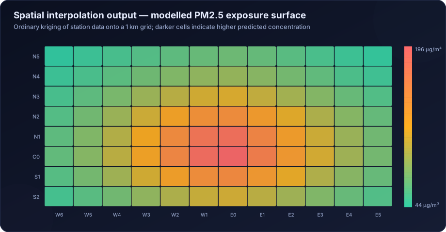
A monitoring station measures concentration at one point. People are distributed across a city and move through it. Assigning a single station's annual mean to an entire district is the simplest approach and often a poor one, especially where the station sits at a traffic hotspot or in an unrepresentative green area.

Methods, in ascending order of rigour

Method	Description	When appropriate
Nearest-station assignment	Everyone gets the nearest monitor's value	Small areas, dense networks, screening
Spatial interpolation	IDW or kriging across monitors to a grid	Moderate network density; see GIS mapping
Land-use regression (LUR)	Statistical model of concentration on land-use, traffic and population predictors	Urban studies with 20+ sites
Dispersion modelling	AERMOD or CALPUFF surfaces from an emission inventory	Project and industrial assessments
Satellite-derived surfaces	AOD converted to surface PM2.5	Large areas, sparse monitoring; see satellite analysis
Hybrid models	Machine learning combining monitors, satellite, land use and meteorology	Best available for national and regional studies
Personal monitoring	Wearable devices on a sample of individuals	Gold standard for exposure validation, expensive

Population weighting

Once a concentration surface exists, exposure must be weighted by where people are:

Population-weighted mean = Σ (population in cell i × concentration in cell i) / Σ (population in cell i)

This matters enormously. A city's simple average across monitors may be 70 µg/m³ while its population-weighted mean is 95 µg/m³, because the population is concentrated in the more polluted core. Reporting the unweighted average understates burden substantially.

Indoor exposure and time-activity

People spend the majority of their time indoors. Total personal exposure is:

E = Σ (fraction of time in microenvironment m × concentration in m)

Ambient pollution penetrates indoors with an infiltration factor typically between 0.5 and 0.8 for PM2.5 in naturally ventilated buildings, so indoor concentration of outdoor origin is lower than ambient — but indoor sources, particularly solid-fuel cooking, can dominate total exposure entirely. See indoor air quality analysis.

In Indian household-air-pollution contexts, ignoring the indoor component is not a refinement issue; it can change the answer by an order of magnitude for the exposed subgroup.

Step 2 — Concentration-Response Functions

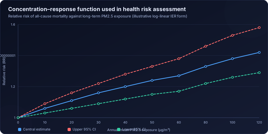
A CRF quantifies how much risk increases per unit of exposure. It is derived from cohort or time-series epidemiological studies, not from the assessment itself.

Short-term versus long-term effects

Short-term (acute) effects come from time-series and case-crossover studies relating daily concentration to daily mortality or hospital admissions. They are typically expressed as a percentage increase in daily events per 10 µg/m³ increase in daily concentration — commonly around 0.5–1.0% per 10 µg/m³ PM2.5 for all-cause mortality.

Long-term (chronic) effects come from cohort studies following populations for years, relating long-term average exposure to mortality. These effects are much larger, typically a 6–8% increase in all-cause mortality per 10 µg/m³ of annual mean PM2.5, and they dominate the total burden.

Do not add them. Short-term and long-term estimates overlap substantially — the deaths brought forward by an acute episode are largely among people already at elevated risk from chronic exposure. Summing the two double-counts. Standard practice is to use long-term functions for total burden and short-term functions separately for episode-specific analysis.

The shape of the function

Early assessments assumed a log-linear relationship — constant proportional risk increase per unit exposure. At the very high concentrations found in Indian cities, this extrapolates far beyond the range of most Western cohort studies and produces implausibly large risks.

The Integrated Exposure-Response (IER) function, developed for the Global Burden of Disease programme, addresses this by fitting a curve across the full global exposure range using evidence from ambient air pollution, household air pollution, second-hand smoke and active smoking. It flattens at high concentrations. Its successor, the Global Exposure Mortality Model (GEMM), is based on cohort studies alone and gives somewhat steeper risks at high exposures.

The choice between them materially changes results for Indian cities, and it must be stated explicitly. Reporting a burden figure without naming the CRF used is not a result.

Where CRFs come from

• The Global Burden of Disease programme at IHME, which publishes the functions used in most national assessments
• The State of Global Air reports from the Health Effects Institute
• The WHO Air Quality Guidelines 2021, which summarise the evidence base underpinning the guideline values
• WHO's HRAPIE and AirQ+ frameworks, which provide functions specifically packaged for health impact assessment
• The India State-Level Disease Burden Initiative published in The Lancet Planetary Health, which is the standard India-specific reference

The counterfactual

Attributable burden is always burden relative to something. Common counterfactuals:

Counterfactual	Value (annual PM2.5)	Interpretation
WHO 2021 guideline	5 µg/m³	Burden relative to the health-based target
WHO interim target 1	35 µg/m³	Burden relative to a nearer-term goal
India NAAQS	40 µg/m³	Burden relative to legal compliance
Theoretical minimum risk (GBD)	2.4–5.9 µg/m³	Burden relative to the lowest observed exposure
Zero anthropogenic	Site-specific natural background	Total anthropogenic burden

The same city produces wildly different burden figures under different counterfactuals. Every burden number must state its counterfactual, and comparisons between studies using different counterfactuals are meaningless.

Step 3 — From Relative Risk to Attributable Burden

The standard calculation chain:

1. Relative risk at the observed exposure

RR = exp(β × (C − C₀)) for a log-linear function, where β is the CRF coefficient, C the observed exposure and C₀ the counterfactual.

2. Population attributable fraction

PAF = (RR − 1) / RR

The PAF is the proportion of cases in the population that would not have occurred at the counterfactual exposure.

3. Attributable cases

Attributable cases = PAF × baseline incidence rate × population at risk

A worked example

Take a district with:

• Population-weighted annual mean PM2.5 = 85 µg/m³
• Counterfactual = 5 µg/m³ (WHO guideline)
• CRF: 8% increase in all-cause mortality per 10 µg/m³ (β = 0.0077 per µg/m³, log-linear, illustrative)
• Baseline all-cause mortality rate = 7.2 per 1,000 per year
• Population = 2,000,000

Calculation:

• RR = exp(0.0077 × 80) = exp(0.616) = 1.85
• PAF = (1.85 − 1) / 1.85 = 0.459, or 45.9%
• Baseline deaths = 7.2/1000 × 2,000,000 = 14,400 per year
• Attributable deaths = 0.459 × 14,400 = 6,610 per year

The result is stark, and it is also an illustration of why the assumptions must be stated. Using the IER function instead of a log-linear extrapolation would reduce this considerably. Using the NAAQS as the counterfactual instead of the WHO guideline would reduce it further. Neither version is "wrong"; they answer different questions.

Step 4 — Beyond Mortality

Comprehensive assessments quantify more than deaths:

Outcome	Typical metric	Data source
Premature mortality	Attributable deaths per year	Vital registration, GBD
Years of life lost (YLL)	Life expectancy at age of death × deaths	Life tables
Disability-adjusted life years (DALY)	YLL + years lived with disability	GBD methodology
Hospital admissions	Respiratory and cardiovascular admissions	Hospital records, short-term CRFs
Emergency visits	Asthma, COPD exacerbation	Health system data
Restricted activity days	Days of limited activity	Survey-based CRFs
Work loss days	Absenteeism	Labour and health surveys
Low birth weight and preterm birth	Attributable cases	Birth registry, specific CRFs
Childhood asthma incidence	New cases attributable to NO2	Cohort-based CRFs

DALYs are the standard for comparing across outcomes and against other risk factors, because they combine mortality and morbidity into a single unit.

Step 5 — Economic Valuation

Converting health burden to monetary terms supports cost-benefit analysis of control measures.

Value of a Statistical Life (VSL) is the standard approach for mortality — the aggregate willingness to pay for a small reduction in mortality risk across a population. It is not the "value of a life"; it is derived from observed trade-offs between money and risk. Country-specific VSL estimates are typically transferred from studies in high-income countries using an income elasticity adjustment.

Cost of illness covers morbidity: treatment costs, medication, lost productivity.

Human capital approaches value lost output rather than willingness to pay and give substantially lower figures.

Economic valuation is the most contested part of health risk assessment, and the sensible presentation is a range across methods with the assumptions visible, not a single headline figure.

Uncertainty: The Part That Must Not Be Omitted

Uncertainty enters at every stage:

• Exposure — spatial model error, station representativeness, indoor infiltration assumptions
• CRF — the confidence interval on the epidemiological coefficient, and the choice of functional form
• Transferability — whether a CRF derived in North American or European cohorts applies at Indian exposure levels and in Indian populations
• Baseline health data — under-registration of deaths and misclassification of cause
• Population data — census currency and spatial disaggregation
• Counterfactual choice

The minimum acceptable treatment is to propagate the CRF confidence interval through to the burden estimate and report a range. Better practice is a Monte Carlo simulation sampling from distributions for exposure, CRF and baseline rates, reporting the median and a 95% credible interval. Best practice adds a structured sensitivity analysis showing how the result changes under alternative CRFs and counterfactuals.

A single point estimate with no interval is the signature of an assessment that has not thought about its own reliability.

Common Errors

• Adding short-term and long-term effects, double-counting the burden.
• Using unweighted station averages instead of population-weighted exposure, typically understating burden.
• Log-linear extrapolation far beyond the CRF's evidence range, inflating risks at high Indian concentrations.
• Omitting the counterfactual from the reported result, making it uninterpretable.
• Ignoring indoor exposure where household solid-fuel use is prevalent.
• Presenting point estimates without uncertainty.
• Interpreting attributable deaths as identifiable individuals. Attributable burden is a population-level statistical construct, not a count of specific people.
• Comparing burden figures across studies that used different CRFs, counterfactuals or exposure methods.

How DSTechnoverse Helps

DSTechnoverse conducts air quality health risk assessments for city programmes, industrial projects, EIA health chapters and research studies.

• Exposure assessment — population-weighted exposure surfaces built from monitoring networks, land-use regression, dispersion modelling or satellite-derived products, integrated with gridded population data in GIS.
• CRF selection and application — appropriate functions chosen for the exposure range and outcome, with the choice justified and the alternatives tested in sensitivity analysis.
• Burden quantification — attributable deaths, YLL, DALYs, hospital admissions and morbidity outcomes, calculated with documented baseline health data and population inputs.
• Uncertainty analysis — Monte Carlo propagation across exposure, CRF and baseline uncertainty, reported as credible intervals rather than point estimates.
• Scenario analysis — burden avoided under specified control scenarios, which is what actually supports investment decisions.
• Economic valuation — VSL and cost-of-illness approaches presented as a transparent range.
• Reporting — methods, data sources, assumptions and limitations documented to the standard expected in peer review and regulatory scrutiny.

Where the assessment supports a project rather than a city, we link it to dispersion modelling so that incremental exposure from the project is quantified on the same basis as the existing background.

---

Need air quality data turned into a defensible answer? DSTechnoverse provides end-to-end air quality analysis services — monitoring data validation, statistical analysis, source apportionment, dispersion modelling, GIS mapping, and regulator-ready reporting. Talk to our air quality team about your dataset or project.

Frequently Asked Questions

What is an air quality health risk assessment?

It is an analysis that quantifies the health burden attributable to air pollution, combining an exposure estimate for a defined population with epidemiologically derived concentration-response functions, baseline disease rates and population data. The output is a number of attributable cases — deaths, hospital admissions or DALYs — relative to a stated counterfactual exposure.

What is a concentration-response function?

It is the relationship between pollutant exposure and the increase in risk of a health outcome, derived from epidemiological studies. It is typically expressed as a percentage increase in risk per 10 µg/m³ of exposure, and it is an input to a health risk assessment rather than something the assessment estimates itself.

What is the population attributable fraction?

The proportion of cases of a health outcome in a population that would not have occurred if exposure had been at the counterfactual level. It is calculated as (RR − 1) / RR, where RR is the relative risk at the observed exposure, and multiplying it by baseline cases gives attributable cases.

Why does the counterfactual matter so much?

Because attributable burden is always burden relative to some alternative exposure. Using the WHO guideline of 5 µg/m³ produces a much larger burden than using India's NAAQS of 40 µg/m³, for the same city and the same data. A burden figure without a stated counterfactual cannot be interpreted or compared.

Can short-term and long-term health effects be added together?

No. The two estimates overlap substantially, because deaths brought forward during an acute episode occur largely among people already at elevated risk from chronic exposure. Adding them double-counts. Long-term functions are used for total burden, and short-term functions are applied separately for episode analysis.

How is exposure estimated for a whole population?

Through a concentration surface — from spatial interpolation, land-use regression, dispersion modelling, satellite-derived estimates or a hybrid model — combined with gridded population data to compute a population-weighted mean. Where indoor sources are significant, time-activity patterns and infiltration factors are needed to estimate total personal exposure.

Do attributable deaths refer to identifiable individuals?

No. Attributable burden is a population-level statistical estimate of how many fewer cases would have occurred at a lower exposure. It cannot identify which individuals were affected, and describing it as though it counts specific people misrepresents what the method produces.

How should uncertainty be reported in a health risk assessment?

At minimum by propagating the concentration-response function's confidence interval to produce a range around the burden estimate. Better practice uses Monte Carlo simulation across exposure, CRF and baseline uncertainty to give a credible interval, plus sensitivity analysis showing how results change under alternative functions and counterfactuals.