How to Make AERMOD Isopleth Maps in QGIS for EIA Reports

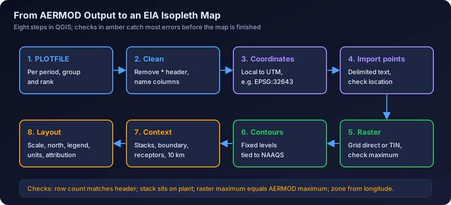
Quick answer: To make an AERMOD isopleth map in QGIS, write the gridded results to a PLOTFILE, convert the receptor coordinates to the correct UTM zone (for example EPSG:32643 for UTM 43N or EPSG:32644 for UTM 44N), import the file as a delimited text layer, turn the regular receptor grid into a raster, and generate contours with the GDAL contour tool. Then add the sources, plant boundary, sensitive receptors and a 10 km study circle, and finish the layout with a scale bar, north arrow, legend and units.

Isopleth maps are often the first part of an air dispersion study that an appraisal committee member, SPCB officer or proponent looks at. A map in the wrong place, with a misleading colour ramp or no units, can undermine an otherwise sound study.

This is a step-by-step guide to producing those maps in QGIS, the free, open source GIS used widely by Indian EIA consultancies. If you want to know how to read and interpret an AERMOD contour map, see our guide to reading AERMOD output contour maps. If you need to interpolate ambient monitoring data across a region, which is a different problem with different methods, see air quality GIS mapping and interpolation.

The steps below assume a recent long-term release of QGIS (3.x). Menu names occasionally move between versions, so if a tool is not where described, search for it by name in the Processing Toolbox.

What You Need Before You Start

Item	Where it comes from	Why it matters
AERMOD gridded output (PLOTFILE)	Your AERMOD run, one file per averaging period and source group	The concentration values to be contoured
Receptor grid definition	The RE pathway in the AERMOD input	Tells you whether the grid is regular and what the spacing is
Coordinate reference	Stack coordinates in UTM, or the local origin used	Places the results correctly on the earth
Source locations	Stack table in the emission inventory	Plotted as symbols on the map
Plant boundary	Site layout drawing or KML from the proponent	Context, fence-line receptors and 10 km circle origin
Applicable standard	NAAQS 2009 values for the pollutant and averaging time	To choose meaningful contour intervals

If you have not yet finalised the receptor grid, read dispersion modelling receptor grid design first. Good maps depend on a good grid, and that decision is made before AERMOD is run, not in QGIS.

Step 1: Get Gridded Output From AERMOD

AERMOD can write results in several ways. For mapping, two output pathway options matter.

PLOTFILE writes one row per receptor with the X and Y coordinates, the concentration for the chosen averaging period and rank, the receptor elevation, hill height and flagpole height, the averaging period, the source group and, for grid receptors, the network ID. A PLOTFILE is requested in the OU (output) pathway, naming the averaging period (for example 24, or PERIOD for the long-term average), the source group (usually ALL, or a named group) and the rank (for example FIRST for the highest, or a specific high value), followed by a file name. You can request one PLOTFILE for each combination you want to map.

POSTFILE writes concentrations for every receptor for every averaging period in the run, for example every hour or every day of the year. It is useful for post-processing, such as calculating your own percentiles or exceedance counts, but the files are large and you would normally summarise them before mapping. For most EIA maps, the PLOTFILE is all you need.

Typical maps for an Indian EIA or CTE report:

Map	AERMOD output	Standard it relates to
Maximum 24-hour PM10 increment	PLOTFILE, 24-hour, FIRST high	NAAQS 2009 24-hour PM10: 100 µg/m³
Maximum 24-hour PM2.5 increment	PLOTFILE, 24-hour, FIRST high	NAAQS 2009 24-hour PM2.5: 60 µg/m³
Maximum 24-hour SO2 increment	PLOTFILE, 24-hour, FIRST high	NAAQS 2009 24-hour SO2: 80 µg/m³
Maximum 24-hour NO2 increment	PLOTFILE, 24-hour, FIRST high, with NO2 conversion option	NAAQS 2009 24-hour NO2: 80 µg/m³
Annual average increment	PLOTFILE, PERIOD (or ANNUAL for multi-year)	NAAQS 2009 annual standards
Maximum 1-hour or 8-hour CO	PLOTFILE, 1-hour or 8-hour, FIRST high	CO: 4 mg/m³ (1-h), 2 mg/m³ (8-h)

Note the ranks carefully. Many Indian reports map the highest 24-hour value at each receptor, which is conservative. Whatever rank you choose, the map title and the report text must say which it is. The units in a PLOTFILE follow the model's output units, which are µg/m³ by default for concentration.

Step 2: Understand and Clean the PLOTFILE

A PLOTFILE starts with header lines beginning with an asterisk, recording the AERMOD version, options, averaging period, source group, rank, receptor count and column names. Data lines follow, with values separated by variable numbers of spaces. That header and spacing trip up a direct import, so there are two routes:

1. Clean it first. Open the file in a spreadsheet or text editor, delete the header lines, split the columns on whitespace, add a single header row (for example X, Y, CONC, ZELEV, ZHILL, ZFLAG, AVE, GRP, NETID) and save it as a comma-separated file. This is the most reliable route and gives you a file that is easy to check.
2. Import with whitespace delimiting. In the QGIS Delimited Text dialog, choose a custom or regular expression delimiter that treats one or more spaces as a separator, set the number of header lines to discard, and name the fields manually. This works, but check carefully that columns have not shifted because of the leading spaces on each line.

Whichever route you use, check the row count against the number of receptors stated in the header, and check that the minimum and maximum values match the AERMOD summary tables in the main output file. A mismatch at this stage means something went wrong in the import.

Step 3: Get the Coordinate System Right

This is the step where most map errors happen.

Local Versus UTM Coordinates

AERMOD works in metres on a flat Cartesian plane. Many studies set up the grid with the main stack at the origin (0, 0), so the PLOTFILE X and Y values are offsets in metres from the stack. Others use real UTM eastings and northings throughout. You must know which, because QGIS needs real-world coordinates.

If the model used a local origin, add the stack's UTM easting to every X value and its UTM northing to every Y value before import. You can do this in the spreadsheet or in QGIS with the Field Calculator after import. Keep the original columns so you can check the result.

UTM Zones Across India

India spans several UTM zones. Each zone is 6 degrees of longitude wide, and the zone number is set by the site longitude, not by the state.

Longitude range	UTM zone	EPSG code (WGS 84)	Examples of regions largely in this zone
66°E to 72°E	42N	32642	Kutch and western Gujarat
72°E to 78°E	43N	32643	Most of Gujarat, Maharashtra, western Madhya Pradesh including Indore, Rajasthan, Punjab, Karnataka, Kerala
78°E to 84°E	44N	32644	Eastern Madhya Pradesh, Telangana, Chhattisgarh, eastern Uttar Pradesh, Tamil Nadu
84°E to 90°E	45N	32645	Odisha, Jharkhand, Bihar, West Bengal
90°E to 96°E	46N	32646	Assam, Meghalaya and much of the North East

Zone boundaries cut through states, so always check the actual site longitude. A plant at 77.9°E and one at 78.1°E are in different zones. Projects near a zone boundary are normally kept in one zone throughout, the zone containing the main source, and the choice is recorded in the report.

Use the WGS 84 datum. Older Indian survey data may use the Everest datum, and mixing datums can shift features by hundreds of metres. A boundary drawn in a local site coordinate system must be georeferenced first.

Setting the Project CRS

In QGIS, set the project coordinate reference system to the UTM zone of the site (for example EPSG:32643) under Project Properties. Load all layers in or reproject them to the same CRS. On-the-fly reprojection will display mixed layers together, but contours and buffers should be generated in a projected CRS in metres, never in latitude and longitude degrees.

Step 4: Import the Results as Points

Use Layer, Add Layer, Add Delimited Text Layer. Choose the cleaned CSV, select Point coordinates, set the X and Y fields to easting and northing, and set the geometry CRS to the correct UTM zone. You should see a regular lattice of points. Check that:

• The points are centred on the plant, not in the sea or in another district.
• The spacing looks right (for example 100 m near the plant and 500 m further out if a nested grid was used).
• Styling the points by concentration with a graduated colour shows the highest values near the expected location.

Save the layer as a GeoPackage so the map project does not depend on the CSV.

Step 5: Turn the AERMOD Grid Into a Surface in QGIS

Contours are generated from a continuous surface (a raster). How you build that raster matters more than most people realise.

Why a Regular Receptor Grid Matters

A Cartesian receptor grid with uniform spacing gives you a value at every node of a regular lattice. That is exactly what a raster is. You can convert it to a raster with almost no interpolation, and the contours then reflect the model's results faithfully.

Discrete receptors, such as twenty village locations, are a very different case. They are irregular and sparse, and drawing contours from them means the interpolation algorithm, not AERMOD, decides what happens between villages. Peaks near the plant can be missed completely. Never contour from discrete receptors alone. Use them as labelled points on top of a map contoured from the grid.

Nested grids (fine near the plant, coarser further out) are sensible but not uniform, so either interpolate lightly to the finest spacing or rasterise each nest separately and merge them with the fine grid taking priority.

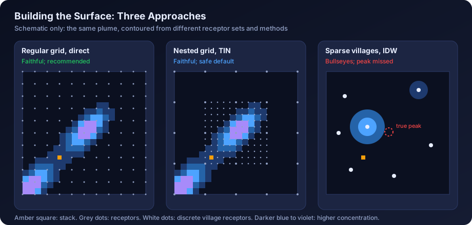
The Three Main Options

Method	QGIS tool	Best for	Watch out for
Use the regular grid directly	Rasterize (vector to raster) with cell size equal to grid spacing, or read a sorted XYZ file as a raster	Uniform Cartesian grids	Cell size and extent must align with the grid nodes exactly
TIN (linear) interpolation	Processing Toolbox, Interpolation, TIN interpolation; or GDAL Grid (Linear)	Nested or slightly irregular grids	Linear between nodes; cannot create peaks higher than the data
IDW interpolation	Processing Toolbox, Interpolation, IDW interpolation	Rarely appropriate for model output	Creates bullseyes around points, flattens peaks, sensitive to power setting
Kriging or splines	Via SAGA or other providers	Monitoring data, not model grids	Can overshoot and invent values above the maximum modelled

For AERMOD results, prefer the regular grid directly, then TIN. TIN is a safe default for nested grids because it honours each node and never exceeds the highest receptor. IDW, designed for scattered observations, produces circular artefacts on gridded data. Kriging is a geostatistical method for sparse monitoring data and is discussed in the GIS interpolation guide; it adds nothing to a dense model grid.

Practical Settings

1. Cell size. Use the finest receptor spacing, or half of it. A finer raster than that adds file size, not information.
2. Extent. Match the receptor grid extent exactly. Do not let the tool extrapolate beyond the outermost receptors.
3. Check the maximum. After building the raster, check its maximum value (Layer Properties, Information). It should equal or be very slightly below the AERMOD grid maximum. If it is higher, the method is overshooting. If it is much lower, the cell size or method is smoothing the peak.

Step 6: Generate Isopleth Contours

With the raster built, use Raster, Extraction, Contour (the GDAL contour tool). Two outputs are useful:

• Contour lines with an attribute for the level, for a clean isopleth map with labels.
• Contour polygons, which fill the bands between levels and make a clearer colour-filled map. Recent QGIS versions include a separate Contour Polygons tool in the GDAL provider.

Use a list of fixed levels rather than a fixed interval. Concentrations fall off steeply with distance, so an interval suited to the peak gives no lines further out, and one suited to the far field produces a dense smudge near the stack.

Choosing Contour Levels Relative to NAAQS

Incremental concentrations from a single project are usually a small fraction of the NAAQS. A useful approach is to set levels as round numbers that also relate to the standard. For example, for 24-hour PM10 (standard 100 µg/m³), levels of 0.5, 1, 2, 3, 5 and 8 µg/m³ correspond to 0.5%, 1%, 2%, 3%, 5% and 8% of the standard, and the legend can show both.

Pollutant and period	NAAQS 2009	Example contour levels for a small increment (µg/m³)	As % of standard
PM10, 24-hour	100 µg/m³	0.5, 1, 2, 3, 5, 8	0.5% to 8%
PM2.5, 24-hour	60 µg/m³	0.3, 0.6, 1.2, 2, 3	0.5% to 5%
SO2, 24-hour	80 µg/m³	1, 2, 4, 6, 8, 12	1.25% to 15%
NO2, 24-hour	80 µg/m³	1, 2, 4, 6, 8, 12	1.25% to 15%
PM10, annual	60 µg/m³	0.1, 0.25, 0.5, 1, 1.5	0.2% to 2.5%

These are illustrative; pick levels that suit your own results. Rules of thumb:

• Aim for five to eight levels per map.
• The lowest level should still be meaningful, not a numerical artefact far from the plant.
• Include at least one level close to the predicted maximum, so the peak area is visible.
• If you map total concentration (increment plus background), say so prominently and draw a contour at the standard itself if it is reached. Most EIA maps show increments only.
• Use the same levels for maps of the same pollutant and period across scenarios, so readers can compare them.

Step 7: Style the Contours Honestly

Colour choice changes how a map is read. Common problems are rainbow ramps that make small differences look dramatic, and red used for levels that are tiny fractions of the standard.

Choice	Recommendation	Reason
Colour ramp	Single-hue or perceptually uniform sequential (light to dark)	Order is clear; no false boundaries
Rainbow ramps	Avoid	Strong hue changes suggest thresholds that do not exist
Red	Reserve for levels near or above a standard, if at all	Red signals danger to most readers
Transparency	40% to 60% for filled bands	Keeps the base map readable
Lowest band	Often left unfilled, or very light	Avoids colouring the whole study area

Label contour lines with their values from the layer styling panel. For filled polygons, use a graduated renderer on the level attribute, darker for higher concentrations. Lightly filled bands with thin labelled lines on top work well.

Step 8: Add Context Layers

A contour map without context is hard to read. Add these layers on top of the contours, and in this order of importance.

1. Sources. Plot every modelled stack with a distinct symbol and a short ID (S1, S2 and so on) that matches the emission table. Area or volume sources, if modelled, should be drawn as their footprint.
2. Plant boundary. Draw the fence line as an outline. Fence-line receptors in the model should sit on or just outside it.
3. 10 km study circle. The EIA study area is commonly a 10 km radius, as set by the ToR or relevant EIA guidance. Create it with Vector, Geoprocessing Tools, Buffer on the plant boundary or main stack (check which the ToR uses), distance 10,000 m, in the UTM CRS. Some reports also draw 2 km and 5 km rings.
4. Sensitive receptors. Villages, schools, hospitals and places of worship identified in the baseline survey, with labels. Use the same names as the receptor table.
5. Ambient monitoring stations. The baseline AAQ locations.
6. Maximum point. Its value, distance and direction from the main stack.

Step 9: Choose a Base Map and Respect Its Licence

Base maps are where copyright and licence questions arise, and EIA reports are public documents.

Source	Typical use	Licence points to check
OpenStreetMap	Roads, settlements, rivers	Open Database Licence; attribution such as "© OpenStreetMap contributors" required
Bhuvan (ISRO)	Indian imagery and thematic layers	Check the terms of use published on the Bhuvan portal
Survey of India Open Series Maps	Topographic context	Check the current terms for use and publication
Commercial satellite imagery services	Imagery backdrop	Many services restrict use outside their own applications, or require a licence and attribution
Imagery you have licensed or captured (for example drone survey)	Site-level detail	Your own licence terms

Do not paste screen captures from web mapping services into a report unless their terms allow it. When in doubt, use OpenStreetMap data or imagery you have licensed, and put the attribution on the map itself.

Step 10: Build the Print Layout

Use Project, New Print Layout. A standard A4 or A3 landscape page works well for most reports.

Add these elements:

• Map frame set to a fixed scale, typically 1:50,000 or 1:75,000 for a 10 km study area on A4. Keep the same scale for all maps of the same study.
• Title stating the pollutant, averaging period, rank, increment or total, and the scenario. For example: "Predicted maximum 24-hour PM10 increment (highest value), proposed expansion, µg/m³".
• Scale bar in kilometres, with round numbers.
• North arrow.
• Legend listing contour levels with units, symbols for sources, boundary, receptors and monitoring stations.
• Coordinate grid or graticule in UTM metres, with the zone stated (for example "WGS 84 / UTM zone 43N").
• Notes box with the model and version, meteorological period, NAAQS for comparison, and data sources and attribution.
• Maximum value annotation: value, location, and distance and direction from the stack.

Export at print resolution (300 dpi is common) as PDF or PNG.

Worked Example: Mapping a Two-Stack Plant in Central India

The following example is illustrative. All numbers are illustrative, to show the method.

A plant near 76.2°E longitude in western Madhya Pradesh has two stacks. The AERMOD run used a local origin at the main stack (S1). S1 is at UTM easting 627,400 m and northing 2,507,800 m in zone 43N. The receptor grid is a nested Cartesian grid: 100 m spacing out to 2 km, and 500 m spacing from 2 km to 10 km. Discrete receptors were placed at 12 villages.

1. Output. PLOTFILEs requested for 24-hour FIRST high and PERIOD averages, source group ALL, for PM10, SO2 and NO2.
2. Cleaning. Header lines removed, columns named, saved as CSV. Row counts checked against the header.
3. Coordinates. Field Calculator used to add 627,400 to X and 2,507,800 to Y. Project CRS set to EPSG:32643, because 76.2°E lies between 72°E and 78°E.
4. Import. Points displayed centred on the plant. A grid receptor near S1 matches the expected location on the base map.
5. Surface. The inner and outer grids were rasterised separately: inner at 100 m cells and outer at 500 m cells, then the outer grid resampled to 100 m and merged with the inner grid taking priority. The raster maximum for 24-hour PM10 is 6.3 µg/m³, matching the AERMOD summary table.
6. Contours. Fixed levels of 0.5, 1, 2, 3, 5 µg/m³ for PM10 24-hour, or 0.5% to 5% of the 100 µg/m³ standard. The 5 µg/m³ contour encloses a small area about 900 m north-east of S1.
7. Context. Stacks S1 and S2, plant boundary, 12 villages, 8 baseline AAQ stations, and a 10 km buffer drawn from the plant boundary as the ToR specifies.
8. Layout. A4 landscape at 1:60,000, light-to-dark single-hue ramp at 50% transparency, labelled lines, OpenStreetMap base map with attribution, UTM grid labelled "WGS 84 / UTM zone 43N", and a note giving the meteorological period and the NAAQS value.

A quick check caught a common error: on the first import, before the offsets were added, the points appeared in the Indian Ocean near the equator. The point layer check in step 4 caught it before any maps were made.

Map Checklist for EIA Reports

Use this checklist before any map goes into a report. It complements the broader QA/QC checklist for air dispersion reports.

Check	Pass condition
Correct location	Sources sit on the plant on the base map
CRS stated	Map shows the datum and UTM zone, for example WGS 84 / UTM zone 44N
Title complete	Pollutant, averaging period, rank, increment or total, scenario
Units	µg/m³ (or mg/m³ for CO) shown in the legend
Raster maximum	Matches the AERMOD output maximum
Contours from grid	Not from discrete receptors alone
Levels sensible	Five to eight levels, related to NAAQS, same across scenarios
Colour ramp	Sequential, not rainbow; red not used for trivial levels
Context layers	Sources, boundary, receptors, AAQ stations, 10 km circle
Maximum marked	Value, distance and direction from main stack
Scale bar and north arrow	Present and correct
Attribution	Base map source and licence stated
Consistency	Values on map match tables in the report

Common Mistakes

• Wrong UTM zone. Using 43N for a site east of 78°E, or the reverse, puts everything hundreds of kilometres away or produces a distorted map. Always calculate the zone from the longitude.
• Local origin not converted. Plotting local X and Y as if they were UTM puts the plant near the zone's false origin, in the Indian Ocean near the equator.
• Interpolating sparse discrete receptors. Contours drawn from a dozen village points are an artefact of the interpolation method, not a model result. Use the grid.
• IDW on a model grid. Produces bullseye rings around every receptor and flattens the peak.
• Misleading colour ramps. Rainbow or red-dominated ramps make a 2 µg/m³ increment look alarming. Use a sequential ramp and show the standard in the legend.
• Units missing or wrong, such as a CO map in µg/m³ compared with a standard in mg/m³.
• Extrapolation beyond the grid, where the model was not run.

Most of these are also on our list of common AERMOD mistakes, which covers modelling set-up errors as well as mapping ones. Getting the inputs right matters just as much: terrain and land use data for AERMOD and the AERMOD input data checklist cover the steps before the run.

How Maps Fit Into the EIA Report

Under the EIA Notification 2006, the ToR for most industrial projects asks for predicted incremental GLCs to be mapped with the baseline monitoring locations, and for increment plus baseline to be compared with NAAQS. The same maps often go into CTE applications to the SPCB. Refer to each map in the text, explaining where the maximum occurs, why, and the values at the nearest sensitive receptors.

For a broader view of report structure, see air dispersion modelling report contents and air dispersion modelling for EIA in India.

How DSTechnoverse Helps

We deliver AERMOD studies with report-ready isopleth maps: receptor grids designed for clean contouring, correct UTM referencing, contour levels tied to NAAQS, licensed base maps and a consistent layout across scenarios. Our AERMOD modelling service supports project proponents and EIA consultancies, including white-label work. If you run your own cases, AERMOD Studio runs the real US EPA AERMOD and AERMET in the browser and produces gridded results ready for GIS. To discuss mapping or modelling support, talk to our team.

Frequently Asked Questions

Which AERMOD output file should I use for contour maps? Use a PLOTFILE for each averaging period, source group and rank you want to map. It contains one row per receptor with coordinates and the concentration, which is exactly what QGIS needs. A POSTFILE holds every receptor for every averaging period and is better suited to post-processing, such as calculating percentiles, before mapping a summary.

Which UTM zone should I use for my site in India? Calculate it from the site longitude: zone 43N covers 72°E to 78°E (EPSG:32643) and zone 44N covers 78°E to 84°E (EPSG:32644). Other parts of India fall in zones 42N, 45N and 46N. Zone boundaries cut through states, so do not assume a zone from the state name. Keep one zone for the whole project.

Should I use IDW or kriging to contour AERMOD results? Usually neither. AERMOD gives values on a dense regular grid, so the best approach is to convert that grid directly to a raster, or use linear TIN interpolation for nested grids. IDW creates bullseye artefacts around points and kriging is designed for sparse monitoring data. Both add assumptions that the model results do not need.

Can I draw contours from discrete village receptors? Not on their own. A handful of irregular points cannot describe the concentration field, and the interpolation method would decide where peaks appear. Model a regular Cartesian grid for contouring and add the village receptors as labelled points on top. Their exact predicted values belong in a table in the report.

What contour levels should I use? Choose five to eight fixed levels as round numbers related to the applicable NAAQS 2009 standard, for example 0.5, 1, 2, 3 and 5 µg/m³ for a 24-hour PM10 increment against a 100 µg/m³ standard. Include a level near the predicted maximum and use the same levels across scenarios so maps can be compared.

Can I use Google satellite imagery as a base map? Check the provider's terms before doing so. Many commercial imagery services restrict use outside their own applications or require a licence and attribution, and an EIA report is a public document. OpenStreetMap data is clearly licensed for reuse with attribution, and Indian sources such as Bhuvan have their own published terms.

Why do my contours appear in the wrong place? The most common causes are a local grid origin that was not converted to UTM, easting and northing swapped, the wrong UTM zone, or a datum mismatch with an older survey drawing. Import the results as points first and check that the main stack sits on the plant before generating any contours.

Should the map show the increment or the total concentration? Most Indian EIA maps show the predicted increment from the project, with total concentrations (increment plus baseline) given in tables at monitoring stations and receptors. If you map totals, say so clearly in the title and legend, explain how background was applied, and consider drawing a contour at the standard itself.

---

Need an AERMOD study or AERMOD software? DSTechnoverse runs regulatory AERMOD modelling studies for EC, CTE and expansion applications, for industries and as a white-label partner for EIA consultancies, and provides AERMOD Studio, our AERMOD software, personalised for your firm. We are based in Indore, Madhya Pradesh and work across India. Talk to our team.