
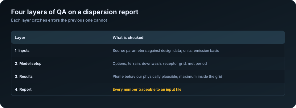
The difference between a study that sails through review and one that bounces back is usually a disciplined QA/QC pass. Whether the modelling was done in-house or by a subcontractor, run this framework before anything reaches a regulator.
Layer 1: Inputs
- Are all source parameters verified against the design basis?
- Is the meteorological data representative, recent, and above the recovery threshold?
- Do surface characteristics match the actual land use, by season and sector?
- Are terrain and elevation processed correctly for the site?
- Is building downwash included where structures warrant it?
Layer 2: Model setup
- Correct model and options for the project (and the terms of reference)?
- Receptor grid fine enough near the source to capture the maximum?
- All required pollutants and averaging periods included?
- Background concentrations added where needed?
Layer 3: Results
- Does the maximum concentration occur at a physically sensible location?
- Are exceedances (if any) plausible given the emission rates?
- Are the correct standards applied to each averaging period?
- Do sensitive receptors show acceptable values?
Layer 4: The report itself
- Is every figure and table traceable to an input or model run?
- Are assumptions and limitations stated clearly?
- Do the maps have scales, legends, and coordinate references?
- Does the narrative match the numbers in the tables?
Make it independent
The most important principle: the person who ran the model should not be the only person who checks it. A second reviewer catches the assumptions the modeller has stopped seeing. If you outsource modelling, confirm your subcontractor performs independent QA before delivery — and still review the output yourself.
Turn it into a template
Convert this framework into a one-page sign-off sheet. Every study gets the same pass, every reviewer looks for the same things, and quality stops depending on who happened to do the work. Consistency is what regulators reward.
Layer 1: inputs, checked against source documents
The reviewer's job at this layer is not to judge whether values are reasonable but to confirm each one matches the document it came from. This is clerical work and it catches the most consequential errors.
| Check | Confirm |
|---|---|
| Stack height | Against the drawing, above grade not above MSL |
| Inner diameter | Inner, not outer; metres not millimetres |
| Exit velocity | Consistent with flow rate divided by area |
| Exit temperature | In kelvin |
| Emission rates | Conversion to g/s reproducible from the original figure |
| Emission basis | Design, permitted or actual — stated |
| Coordinates | One projection across sources, buildings, terrain, receptors |
| Base elevations | Consistent datum for stacks and buildings |
| Operating hours | Match the plant's actual regime |
The internal consistency check on velocity is the most productive single test. Exit velocity, stack diameter and volumetric flow are related, so any two determine the third. If the supplied numbers do not reconcile, one of them is wrong and the whole assessment rests on it.
Have this layer done by someone who did not run the model. A modeller re-reading their own input table sees what they intended to enter.
Layer 2: model configuration
| Check | Confirm |
|---|---|
| Model version | Current, and stated in the report |
| Regulatory default options | Used, or every deviation justified |
| Meteorological period | Full years, with recovery documented |
| Met station | Justified on distance, elevation, terrain, land use |
| Surface characteristics | By sector and season, describing the station's surroundings |
| Terrain | AERMAP run; DEM extends beyond the receptor grid |
| Building downwash | BPIP-PRIME run, or absence justified |
| Receptor grid | Fine near source, extending past the maximum |
| Sensitive receptors | Entered as discrete points at real coordinates |
| Averaging periods | Every period the applicable standards require |
| Urban or rural option | Chosen on population and land use, and justified |
The urban/rural switch is easy to overlook and affects results materially, because urban mode adds heat-island-driven turbulence that keeps the boundary layer mixed at night. Choosing it for a rural industrial site under-predicts night-time concentrations. The choice should be made on land use within 3 km and stated.
Layer 3: results, checked for physical plausibility
| Check | Expected |
|---|---|
| Location of the maximum | Hundreds of metres to a few km for a tall stack |
| Maximum inside the grid | Not on the domain boundary |
| Plume orientation | Consistent with the wind rose |
| Concentration decay with distance | Monotonic, except where terrain intercepts |
| Annual vs short-term ratio | Annual typically 5 to 20 times lower |
| Order of magnitude | Within a factor of a few of a screening estimate |
| Elevated receptors | Higher values where terrain rises into the plume |
| Sensitive receptor values | Consistent with adjacent grid points |
The screening cross-check is the single most valuable test at this layer. Run AERSCREEN, or do a rough hand calculation, and compare. Screening should be conservative — higher than the refined result, but within a factor of a few. A refined result an order of magnitude away from the screening estimate almost always indicates a unit error in the inputs, and it is far better to find that yourself.
Plume orientation is the other quick diagnostic. Contours that do not follow the prevailing wind directions usually mean the wrong met file, or coordinates in the wrong projection.
Layer 4: the report itself
| Check | Confirm |
|---|---|
| Every table reproducible from the input files | The traceability standard |
| Model version and options listed | Including deviations from defaults |
| Met data source, period and recovery stated | With gap treatment |
| Input parameter table included | Full, with units and sources |
| Background concentrations added | With monitoring source, location and period |
| Correct statistic per averaging period | 98th percentile where applicable |
| Compliance conclusion follows from the numbers | Total against limit, not increment |
| Maps legible | Scale, north arrow, receptor labels, contour values |
| Sensitive receptors named | Not "the nearest village" |
| Limitations stated | Model assumptions and data gaps |
| Input files appended or available | So the study can be reproduced |
The traceability standard is the one to hold above all others: another competent modeller, given your input files, should reproduce every number in your report. Where they cannot, the report is not defensible even if the modelling was entirely correct.
Making review independent, and making it a habit
Self-review does not work, for a well-understood reason: you check what you meant to do rather than what you did. The reviewer should be someone who did not run the model, and should work from source documents rather than from the modeller's summary.
Where a team is too small for that, two practices help. Review after a gap of at least a day, so the work is less familiar. And review against a written checklist rather than by general reading, so the check is complete rather than impressionistic.
Turn the four layers into a document with a sign-off line per section, the reviewer's name and the date. Over time it becomes a record of the issues your team actually encounters, and it can be handed to a client or regulator as evidence the study was reviewed. For projects where modelling is subcontracted, the checklist becomes the acceptance criteria — see how to outsource air dispersion modelling.
For the specific failures this process is designed to catch, see 10 common AERMOD modelling mistakes; for reading the outputs, how to read AERMOD output. Our AERMOD air dispersion modelling service applies independent review to every study before delivery. The US EPA modelling guidance sets out the documentation regulators expect.
Frequently Asked Questions
How do I QA an air dispersion modelling report?
In four layers: verify every input against its source document, check the model configuration and options, test the results for physical plausibility against a screening estimate, and confirm the report is traceable — that every number can be reproduced from the input files.
Who should review a dispersion modelling report?
Someone who did not run the model, working from the original source documents rather than the modeller's summary. Self-review reliably misses errors because the reviewer checks what they intended to do rather than what they actually did.
What is the most important QA check?
Confirming that every table in the report can be reproduced from the input files. A study that cannot be reproduced is not defensible regardless of whether the modelling itself was correct.
How do I know if my AERMOD results are plausible?
Compare them against a screening model such as AERSCREEN, or a rough hand calculation. Screening should be conservative but within a factor of a few. An order-of-magnitude difference almost always indicates a unit error in the input data.
What is the urban versus rural option in AERMOD?
A switch that adds heat-island-driven turbulence to keep the night-time boundary layer mixed. It should be chosen on land use within about 3 km of the source and stated in the report — using urban mode at a rural site under-predicts night-time concentrations.
Should input files be included with the report?
Yes, either appended or made available on request. Regulators increasingly expect it, and it is the practical expression of the traceability standard that any competent modeller should be able to reproduce your results.
Need a modelling or EIA data desk without the overhead? DSTechnoverse works as a confidential, white-label subcontractor for air and water dispersion modelling and EIA data analysis. Get in touch to scope your next project.