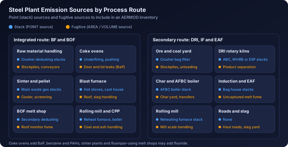
Quick answer: Air dispersion modelling for a steel plant in India means building an AERMOD model of every significant stack (sinter, pellet, coke oven, blast furnace, BOF, DRI kiln, furnaces, power plant) and every material fugitive source (stockyards, transfer points, roads, coke oven tops, slag and char handling), with building downwash for the large shop buildings. The predicted increments for PM10, PM2.5, SO2, NOx, CO and, where coke ovens exist, benzo(a)pyrene are added to measured baseline and compared with NAAQS 2009. In steel clusters the cumulative case, including neighbouring units, usually decides whether the study holds up at appraisal.
Steel is one of the most demanding sectors for an air quality impact assessment. A single integrated works can have more than fifty emission points, several of them at ground level, spread over a site several kilometres across, with buildings large enough to drag plumes down to the ground. A secondary steel unit is smaller, but it often sits in a cluster where a dozen similar plants share the same air shed and the same monitoring stations. In both cases the EAC or SEAC wants to see that the modeller understood the process, not just the stack list.
This guide covers the Indian steel process routes, their sources and pollutants, emission data, AERMOD setup for stacks, fugitives and buildings, cumulative impact in clusters, and a worked expansion example, for teams preparing Environmental Clearance (EC) or Consent to Establish (CTE) applications.
Steel Process Routes in India and Why They Matter for Modelling
India produces steel by two broad routes, and the emission profile of each is very different. Getting the route right at the scoping stage decides which pollutants you model, which sources dominate, and how much of the impact comes from low-level fugitives.
The Integrated Route: Blast Furnace and Basic Oxygen Furnace
The integrated route starts with iron ore and coking coal. The main units are:
- Raw material handling and stockyards: ore, coking coal and flux received by rail or conveyor and stacked in open or covered yards.
- Coke ovens and by-product plant: emissions from the underfiring stack, charging, pushing, quenching, and leaks from doors, lids and offtakes.
- Sinter plant: the main waste gas stack after the wind box ESP is one of the largest point sources on site, with plant dedusting for the cooler and screens.
- Pellet plant: the indurating machine stack emits PM, SO2 and NOx depending on fuel and ore.
- Blast furnace: hot stove stacks burning blast furnace gas, plus cast house and stockhouse dedusting.
- Basic oxygen furnace (BOF): primary off-gas is recovered or flared; secondary emissions go to a dedusting stack.
- Rolling mills: reheating furnace stacks, plus lime kilns and captive power plants.
For modelling, the integrated route produces a large number of tall, high-flow point sources, plus a significant fugitive load from material handling and coke ovens.
The Secondary Route: DRI, Induction Furnace and Electric Arc Furnace
India has an unusually large secondary steel sector, much of it based on coal-based direct reduced iron (sponge iron). A typical secondary unit includes:
- Coal-based DRI rotary kilns: off-gas passes through a dust settling chamber and an after burning chamber (ABC), then a waste heat recovery boiler (WHRB) or gas conditioning tower, an ESP and a stack. Product separation and char handling are dusty.
- Induction furnaces: fume extraction hoods and bag filters; hood capture efficiency is often the weak point.
- Electric arc furnaces: fourth-hole extraction plus canopy hood, ducted to bag houses.
- Rolling mills with gasifier or oil-fired reheating furnaces.
- Captive power plants: WHRBs on DRI kiln heat, often with an AFBC boiler firing coal, washery rejects or char (dolochar).
The secondary route has fewer stacks but more uncertain emission data, more fugitive dust per tonne of product, and a strong tendency to cluster geographically. Modelling these units well depends on realistic fugitive estimates and an honest cumulative assessment.
Sources and Pollutants: What to Model
The pollutants in the ToR for a steel project are normally PM10, PM2.5, SO2, NOx (reported against the NO2 standard) and CO. Where coke ovens are present, benzo(a)pyrene, benzene and other PAHs become important, and fluoride may be raised for sinter plants and some steel melt shops that use fluorspar. The table below summarises the main sources and their typical pollutants.
| Unit | Main point sources | Main fugitive sources | Key pollutants |
|---|---|---|---|
| Raw material handling | Dedusting stacks at crushers and junction houses | Stockpiles, stacker-reclaimers, wagon tipplers, conveyor transfers | PM10, PM2.5 |
| Coke ovens | Underfiring stack, pushing emission control stack | Door, lid and offtake leaks; charging; quenching | PM, SO2, NOx, CO, BaP, benzene, PAHs |
| Sinter plant | Main waste gas stack, plant dedusting stack | Cooler discharge, sinter handling | PM, SO2, NOx, CO, fluoride (ore dependent) |
| Pellet plant | Indurating machine stack, dedusting stacks | Fines handling, pellet screening | PM, SO2, NOx |
| Blast furnace | Hot stove stack, cast house and stockhouse dedusting | Cast house roof (uncaptured), slag handling | PM, SO2, NOx, CO |
| BOF / steel melt shop | Secondary dedusting stack | Shop roof monitor during charging and tapping | PM, CO, fluoride (if fluorspar used) |
| DRI kiln | ABC, WHRB or ESP stack | Product separation, cooler discharge, char and coal handling | PM, SO2, NOx, CO |
| Induction / electric arc furnace | Fume extraction bag house stack | Uncaptured melting fumes through building openings | PM, CO |
| Rolling mill | Reheating furnace stack | Minor | PM, SO2, NOx |
| Captive power plant | Boiler stack | Fly ash and coal handling | PM, SO2, NOx |
A few points that experienced reviewers check:
- SO2 is fuel and ore driven. Sinter plants, pellet plants, coke oven underfiring and coal-fired captive boilers dominate SO2. DRI kilns emit SO2 from the sulphur in non-coking coal, and the share captured in the product or char varies.
- CO is not trivial. Blast furnace gas and DRI kiln off-gas are rich in CO before combustion. A failed ABC, a bleeder opening or an unburnt flare can produce short-term CO peaks, and the NAAQS for CO are 1-hour and 8-hour values (4 mg/m³ and 2 mg/m³).
- BaP is a long-term issue. The NAAQS for benzo(a)pyrene is an annual value of 1 ng/m³. Coke oven battery top emissions are low-level and diffuse, so the annual impact concentrates near the battery. This is often the parameter that needs the most careful explanation.
- Fluoride is not a NAAQS parameter in India, so if it is raised in the ToR, explain the basis for any comparison (for example a vegetation or occupational reference) rather than presenting it as a compliance test.
For a general explanation of these parameters and their health relevance, see air quality parameters explained, and for the standards themselves see NAAQS standards in India explained.
Stack Versus Fugitive Emissions
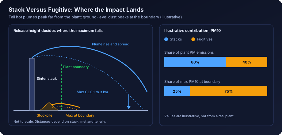
The single most common weakness in steel plant models is treating the plant as a list of stacks. Stacks usually carry the larger mass of SO2 and NOx, but fugitive sources often carry a large share of PM and almost all of the near-field PM impact.
The reason is release height. A sinter main stack may release at well over 100 m with a hot, high-volume plume that rises further. A stockpile releases at ground level with no plume rise at all. A gram per second from the stockpile can produce a near-field concentration many times higher than a gram per second from the tall stack. In AERMOD terms, low-level area and volume sources dominate the receptors at and just beyond the boundary, while the tall stacks dominate the maximum somewhere further out, typically one to a few kilometres away depending on stability and stack parameters.
How to Represent Each Type in AERMOD
| Source | AERMOD source type | Notes |
|---|---|---|
| Process stacks and dedusting stacks | POINT | Use actual exit temperature and velocity, and the stack inner diameter at exit |
| Rain-capped or horizontal vents | POINTCAP or POINTHOR | Only where the stack truly has a cap or horizontal release |
| Stockpiles and open yards | AREA or AREAPOLY | Wind-dependent emission factors; consider hourly variation with wind speed |
| Conveyor transfer points, crushers without dedusting | VOLUME | Initial lateral and vertical dimensions from the structure size |
| Shop roof monitors (cast house, melt shop) | VOLUME or line of volumes, or BUOYLINE where appropriate | Uncaptured fraction only; avoid double counting with dedusting stacks |
| Coke oven battery top | AREA or VOLUME (or line of volumes along the battery) | Release height near battery top; low buoyancy assumed unless justified |
| Haul roads | LINE or a series of VOLUME sources | Silt loading and vehicle data drive the emission rate |
Wherever possible, base fugitive emission rates on a documented method such as US EPA AP-42 emission factors for aggregate handling, wind erosion and paved or unpaved roads, adjusted for the control measures actually committed (water sprinklers, covered conveyors, wind barriers, enclosed sheds). State the control efficiency you assumed and why. The emission inventory for dispersion modelling guide covers the general approach.
Emission Data Sources for a Steel Plant Model
Reviewers will ask where every number came from. For an existing plant being expanded, and for a new plant, the hierarchy below is a sensible one.
Existing Units
- Continuous emission monitoring systems (CEMS): CPCB directions require online monitoring for highly polluting industries including iron and steel, with data linked to the CPCB and SPCB servers. CEMS gives concentration time series for PM and, at many stacks, SO2 and NOx. Use it to establish typical and high percentile concentrations, but check the data quality: calibration records, flatlined periods and outages.
- Periodic stack monitoring reports: third-party or SPCB monitoring with measured velocity, temperature, flow and concentration. These provide the flow data that CEMS concentration alone does not.
- Environmental statements and consent compliance reports: useful cross-checks on stack inventory and production levels.
The stack emission monitoring data analysis guide explains how to turn raw monitoring into defensible modelling inputs, including how to treat values below the detection limit and how to normalise to oxygen or reference conditions.
New Units and Expansions
- Supplier design data: stack gas flow, exit temperature, diameter and the guaranteed outlet concentration of the ESP or bag filter.
- CPCB industry-specific emission standards: the Environment (Protection) Rules set standards for integrated iron and steel plants, sponge iron plants, coke ovens and furnace types, covering particulate matter and, for several units, SO2, NOx and other parameters. New stacks are often modelled at the standard limit, or at a lower vendor guarantee the proponent will accept as a consent condition. Check the latest notification, as these standards have been revised over time.
- Mass balance: for SO2, a sulphur balance on coal, coke, ore and flux, with stated retention in slag, char or product.
- Emission factors: AP-42 and EMEP/EEA factors for fugitive sources and cross-checks, with site-specific activity data.
Most steel ToRs need at least an existing and a post-expansion scenario, often with a third mitigation scenario. Keep source names identical across scenarios so reviewers can see what changed.
Building Downwash in Large Plant Complexes
Steel plants have some of the largest industrial buildings in the country: blast furnace cast houses, BOF shops, rolling mill sheds that may be several hundred metres long, sinter buildings and power plant boiler houses. Many stacks are short relative to these buildings, especially dedusting stacks and reheating furnace stacks that sit beside or on top of the shop.
The rule of thumb that a stack below about 2.5 times the height of a nearby building can be affected by downwash means that a 40 m dedusting stack beside a 35 m melt shop is almost certainly in the wake. AERMOD handles this through the PRIME algorithm with building dimensions prepared by BPIP-PRIME. For a steel plant this means:
- Digitising outlines and tier heights for every significant structure, with tiered structures such as a BF and its cast house as separate tiers.
- Checking very long buildings, because a rolling mill shed can produce large projected widths for some wind directions.
- Running a sensitivity case with and without downwash to show where it matters.
The AERMOD building downwash and BPIP guide covers the mechanics. Downwash often explains why a predicted maximum sits close to the plant boundary.
Meteorology, Terrain and Receptors
Steel plants in India sit in very different settings: flat alluvial plains in parts of West Bengal and Jharkhand, rolling plateau terrain around Raipur and Raigarh, hilly ground near Angul, Keonjhar and Bellary, and coastal locations on the eastern seaboard.
- Meteorology: hourly surface and upper-air data processed by AERMET; see meteorological data for air modelling in India.
- Terrain: in hilly areas elevated receptors can intercept plumes from tall stacks, so AERMAP processing is essential; see terrain and land use data for AERMOD.
- Receptors: a nested grid, close boundary spacing, and discrete receptors at monitoring stations and villages; see receptor grid design. Fugitive sources create steep gradients at the fence line, so a coarse grid can miss the maximum entirely.
Cumulative Impact in Steel Clusters
Secondary steel units in particular are concentrated in clusters. Well-known examples include the industrial belts around Raipur (Siltara and Urla), Raigarh, Durgapur and the wider Asansol area, Angul and Jharsuguda in Odisha, Bellary-Hospet in Karnataka, and parts of Jharkhand. In these areas the baseline air quality already reflects many neighbouring plants, and SPCBs and the EAC increasingly ask for an explicit cumulative assessment.
A practical approach is:
- Identify neighbouring sources in the study area from consent lists, EC records and site visits.
- Avoid double counting. Measured baseline already includes operating neighbours. What it excludes is anything approved but not yet operating, and the project expansion.
- Model committed sources with the expansion and add the result to the measured baseline, at monitoring stations and at the predicted maximum.
- Discuss hotspots honestly. If the baseline is already near the 24-hour PM10 standard, a small increment still matters.
The cumulative air quality impact assessment in India guide sets out the method in detail, including how to handle the 98th percentile form of the 24-hour standards.
Regulatory Context for Steel Projects
Steel projects fall under the metallurgical industries (ferrous) item of the EIA Notification 2006, appraised by the EAC or SEAC depending on category, with expansions also reporting compliance with earlier EC conditions. The ToR typically asks for one season of baseline monitoring (excluding monsoon), prediction of incremental ground level concentrations with site-specific meteorology, isopleths, a table of baseline plus increment against NAAQS 2009, and details of stack and fugitive controls. At the consent stage, the SPCB grants CTE on the same inventory, so the modelled stack parameters effectively become commitments. The air quality modelling for environmental clearance guide covers the overall ToR expectations, and stack height calculation per CPCB guidelines explains the stack height formulas that apply alongside the modelling.
Worked Example: Secondary Steel Unit Expansion
The following example is illustrative. The numbers are chosen to show method, not to represent any real plant or any regulatory limit.
The Project
An existing secondary steel unit operates 2 coal-based DRI kilns of 100 TPD each, 2 induction furnaces, a rolling mill and an 8 MW WHRB power plant. It proposes to add 2 DRI kilns of 350 TPD each, a new induction furnace and ladle refining furnace, a continuous casting machine, and a 30 MW captive power plant (WHRB plus AFBC firing coal and char).
Step 1: Build the Source Inventory
| Source (illustrative) | Height (m) | Exit temp (K) | Exit velocity (m/s) | PM (g/s) | SO2 (g/s) | NOx (g/s) |
|---|---|---|---|---|---|---|
| Existing DRI kilns, common stack | 45 | 430 | 15 | 1.2 | 3.0 | 1.0 |
| New DRI kilns, WHRB stacks (2 sources) | 65 | 420 | 16 | 1.8 each | 5.5 each | 2.0 each |
| AFBC boiler stack | 80 | 410 | 18 | 1.5 | 6.0 | 4.0 |
| Induction furnace bag house stacks (3) | 30 | 340 | 14 | 0.3 each | negligible | negligible |
| Rolling mill reheating furnace | 35 | 480 | 10 | 0.2 | 0.8 | 0.6 |
| Raw material yard (AREAPOLY) | 0 to 2 | ambient | n/a | 0.9 | none | none |
| Product separation and char handling (VOLUME) | 8 | ambient | n/a | 0.4 | none | none |
| Internal roads (series of VOLUME) | 2 | ambient | n/a | 0.6 | none | none |
PM10 is assumed equal to total PM for stacks with bag filters and ESPs, and a PM2.5 fraction is applied by source type using documented particle size fractions. Fugitive rates already include the committed controls (dry fog at transfer points, wind barriers on two sides of the yard, regular road sweeping and sprinkling).
Step 2: Set Up the Model
- Process one year of hourly meteorology through AERMET, using site-representative surface data and upper-air data, with land use characteristics for the area around the met station.
- Run AERMAP with SRTM or better elevation data, since the site is on gently undulating ground with a ridge about 6 km to the east.
- Run BPIP-PRIME with the induction furnace shed, the DRI kiln structures, the WHRB buildings and the power plant boiler house.
- Define a nested receptor grid (50 m spacing near the boundary, 100 m to 2 km, 250 m to 5 km, 500 m to 10 km), boundary receptors at 25 m, and discrete receptors at the 8 baseline monitoring locations.
- Run the existing and post-expansion scenarios with regulatory default options. For NO2, use a documented conversion approach (for example ARM2 or the ozone limiting method if hourly ozone data are available) and state it.
Step 3: Review the Results
| Parameter (illustrative) | Max baseline at monitoring stations (µg/m³) | Predicted max increment, post-expansion (µg/m³) | Location of max increment | Resultant (µg/m³) | NAAQS (µg/m³) |
|---|---|---|---|---|---|
| PM10, 24-h | 82 | 9.5 | 300 m north of boundary | 91.5 | 100 |
| PM2.5, 24-h | 44 | 4.1 | 300 m north of boundary | 48.1 | 60 |
| SO2, 24-h | 18 | 11.2 | 1.6 km east, rising ground | 29.2 | 80 |
| NO2, 24-h | 24 | 6.3 | 1.8 km east | 30.3 | 80 |
Note that adding the maximum increment to the maximum baseline is conservative, because the two maxima are rarely at the same place. Many reports present both this conservative sum and the paired value at each monitoring location.
Step 4: Interpret
Three findings stand out in this illustrative case:
- PM10 is driven by fugitives. Source contribution analysis shows that around two-thirds of the maximum 24-hour PM10 increment near the north boundary comes from the raw material yard, char handling and roads. The new tall stacks contribute little at that receptor.
- SO2 is driven by the new stacks and terrain. The maximum SO2 increment sits on the rising ground to the east, where plumes from the 65 m and 80 m stacks meet elevated terrain under stable conditions. Running the case in flat terrain would have placed the maximum at a lower value closer to the plant.
- The PM10 resultant is close to the standard. With a resultant of about 92 µg/m³ against 100, the reviewer will ask for a mitigation scenario and for the cumulative case with committed neighbouring units.
Mitigation Scenarios
A mitigation scenario shows the committee that the proponent has options and that the predicted impact is not the best that can be done. For steel plants, the measures that usually make a measurable difference in the model are:
| Measure | Effect in the model | Typical pollutant benefit |
|---|---|---|
| Enclosing raw material and char yards, or adding wind barriers | Lower fugitive emission rate through wind erosion and handling factors | PM10 and PM2.5 near the boundary |
| Dry fog or water spray at transfer points, covered conveyors | Lower VOLUME source emission rates | PM near the plant |
| Paving and mechanised sweeping of internal roads | Lower silt loading, lower road emission rate | PM near the plant |
| Improved hood capture at induction furnaces | Shift from uncaptured building release to captured stack release | PM near the plant |
| Raising stack height to meet or exceed CPCB formula values | Higher effective release, lower near-field impact | SO2, NOx, PM |
| Lower outlet concentration from ESP upgrade or bag filter | Lower point source emission rate | PM |
| Low-sulphur coal or FGD / dry sorbent injection | Lower SO2 emission rate | SO2 |
| Green belt along the boundary | Usually not modelled as a removal mechanism; describe qualitatively | Visual and local benefit |
In the illustrative example, enclosing the raw material yard and paving internal roads reduces the maximum 24-hour PM10 increment from 9.5 to about 5 µg/m³. Presenting this as a committed package is far stronger than a generic list of good practices.
EC Expansion Studies: What Reviewers Ask
Steel expansion proposals get a predictable set of queries. Preparing for them at the modelling stage saves a round of additional information requests.
- Does the existing plant model explain the baseline? High measured PM10 with a near-zero modelled contribution suggests missing fugitive sources.
- Are all stacks in the inventory? Cross-check the consent order and environmental statement. Missing dedusting stacks are common.
- Are emission rates at consented limits or measured levels? Either can be justified, but state which and why.
- Has building downwash been considered? For steel plants, it should be.
- Has the cluster's cumulative impact been assessed? Especially in critically polluted areas.
- What are the BaP and benzene impacts? Where coke ovens are involved.
- What do the mitigation measures achieve? A with and without comparison is the clearest answer.
For a fuller checklist of mistakes, see common AERMOD mistakes, and for how the results should be laid out in the report, see air dispersion modelling report contents.
Two practical habits help: use source groups (existing stacks, new stacks, fugitives) so contribution analysis is straightforward, and overlay contours on a base map with villages and monitoring stations, as explained in reading AERMOD output contour maps. For a large captive power plant, the thermal power plant modelling guide covers the boiler side, and the mining projects guide covers captive iron ore mines.
How DSTechnoverse Helps
DSTechnoverse prepares AERMOD studies for steel plants and secondary steel units, covering point and fugitive source inventories, BPIP-PRIME building downwash, AERMET meteorology, terrain processing, cumulative cluster scenarios and mitigation cases, written up in a format that EIA consultants can drop into their reports. We also work white-label for EIA consultancies. Explore our AERMOD modelling service, or if your team prefers to run screening cases in-house, our browser-based AERMOD Studio handles point sources in flat terrain. To discuss a project, talk to our team.
Regional guides: for local regulators, industrial areas and meteorological data in steel clusters, see AERMOD modelling in Odisha and Chhattisgarh, Bengaluru and Karnataka and Gujarat.
Frequently Asked Questions
Which pollutants must be modelled for a steel plant EC study in India? The ToR normally specifies PM10, PM2.5, SO2, NOx and CO, compared with NAAQS 2009 after adding the measured baseline. Where coke ovens are part of the project, benzo(a)pyrene and benzene are usually added, and fluoride may be requested for sinter plants or melt shops using fluorspar. Always follow the exact ToR issued for the project.
Do fugitive emissions really need to be modelled for a steel plant? Yes. Fugitive sources such as stockyards, transfer points, roads, char handling and coke oven tops release at or near ground level, so they often dominate PM10 and PM2.5 concentrations near the plant boundary. A stack-only model will usually underpredict near-field impact and fail to explain the measured baseline, which reviewers notice.
How are coke oven battery emissions represented in AERMOD? The underfiring and pushing emission control stacks are POINT sources. Leaks from doors, lids and offtakes are usually represented as an area source or a line of volume sources along the battery top, with release height near the top of the battery. Emission rates come from leakage-based estimates or emission factors, adjusted for the control system installed.
Is building downwash important in steel plants? Usually it is. Cast houses, melt shops, rolling mill sheds and boiler houses are tall and large, and many dedusting and furnace stacks are not much higher than these buildings. AERMOD's PRIME algorithm with BPIP-PRIME building inputs is the standard approach, and ignoring downwash can understate near-field concentrations from medium-height stacks.
What emission rate should be used for new stacks? For a new unit there is no measured data, so the usual choice is the CPCB emission standard for that unit type or the supplier's guaranteed outlet concentration if it is lower and the proponent will accept it as a consent condition. Combine the concentration with the design gas flow to get a mass emission rate in g/s.
How is cumulative impact handled in a steel cluster? Measured baseline already includes operating neighbours, so they are not added again. The model should include the project expansion and any nearby units that are approved but not yet operating. The modelled increment is then added to the baseline at each monitoring location and at the predicted maximum, and compared with NAAQS.
Can AERMOD handle short-term CO peaks from blast furnace or DRI operations? AERMOD can model 1-hour and 8-hour CO averages directly. Normal operation is modelled with steady emission rates, while upset events such as bleeder openings or ABC failures are usually discussed qualitatively or as a separate emergency scenario, because they are not continuous and are controlled through operating procedures rather than design.
Does terrain matter for steel plants? It matters wherever the terrain around the plant rises to a height comparable with the effective plume height, which is common near Angul, Keonjhar, Bellary and parts of Chhattisgarh. Elevated receptors can receive higher concentrations from tall stacks under stable conditions. AERMAP terrain processing should be used unless the area is demonstrably flat.
Can a small secondary steel unit use simpler modelling? The method is the same, but the scale is smaller. A unit with a handful of stacks and modest fugitive sources can still need downwash, a fine boundary grid and a cumulative case if it sits in a cluster. Simplification usually comes from fewer sources, not from skipping steps that reviewers expect.
Need an AERMOD study or AERMOD software? DSTechnoverse runs regulatory AERMOD modelling studies for EC, CTE and expansion applications, for industries and as a white-label partner for EIA consultancies, and provides AERMOD Studio, our AERMOD software, personalised for your firm. We are based in Indore, Madhya Pradesh and work across India. Talk to our team.