Stack Emission Monitoring Data Analysis: CEMS, Isokinetic Sampling and Compliance

Ambient monitoring tells you what is in the air. Stack monitoring tells you what a facility put there. The two are complementary, and the source side is the one where the numbers are legally binding, financially consequential, and — because of the corrections involved — most frequently miscalculated. A stack concentration reported without oxygen correction, moisture basis and temperature reference stated is not a compliance number; it is an uninterpretable one.

This guide covers stack emission data analysis in full: how CEMS and manual sampling work, the corrections that must be applied and why, how emission rates are derived, how excursions are analysed, and how source data becomes both compliance evidence and the input to dispersion modelling.

Stack emission monitoring data analysis is the validation, correction and interpretation of pollutant measurements taken at an emission source. It covers Continuous Emission Monitoring System (CEMS) data validation and availability assessment, correction of measured concentrations to standard temperature, pressure, moisture and reference oxygen conditions, calculation of mass emission rates, statistical assessment against consent limits, and use of the resulting emission factors in inventories and dispersion models.

Two Measurement Regimes

Continuous Emission Monitoring Systems (CEMS)

A CEMS measures pollutant concentration in the flue gas continuously. Two architectures:

Extractive systems draw a sample from the duct through a heated line to analysers in a shelter. Hot-wet extractive keeps the sample above dew point and measures on a wet basis; cool-dry systems condition the sample and measure dry. The distinction matters because it determines whether a moisture correction is required.

In-situ systems measure across the duct or at a probe within it, with no sample transport. Cross-duct systems give a path-averaged concentration, which handles stratification well.

Measurement principles are typically NDIR or FTIR for SO2, CO and CO2; chemiluminescence or NDUV for NOx; paramagnetic or zirconia for O2; opacity or beta attenuation and light scattering for particulate. Flow is measured by pitot array, ultrasonic transit time, or thermal mass.

Under Indian regulation, CEMS installation is mandatory for a defined list of highly polluting industries, with data transmitted to the SPCB and CPCB servers. The regulatory framework sits with CPCB.

Manual stack sampling

Periodic sampling by a trained team following prescribed methods. Particulate sampling must be isokinetic — the sample is drawn at exactly the velocity of the flue gas at the sampling point. If the sampling velocity is too low, the gas streamlines diverge around the nozzle and heavier particles carry into it, over-sampling coarse particulate; too high, and the opposite occurs.

Isokinetic sampling requires a preliminary velocity traverse to map the velocity profile, sampling at multiple points across two perpendicular diameters, and continuous adjustment of the sampling rate as conditions change. Acceptable isokinetic ratio is generally 90–110%; outside that band the sample is invalid regardless of how carefully the laboratory analysed it.

The reference methods are the US EPA Method 1 through 5 series (traverse points, velocity, molecular weight, moisture, particulate) documented at EPA's Emission Measurement Center, with corresponding Indian standards under the IS series.

The Corrections: Where Most Errors Live

A raw stack concentration is meaningless without stating the basis. Four corrections apply.

1. Standard temperature and pressure

Gas volume changes with temperature and pressure, so concentrations are normalised to standard conditions — typically 0°C (273 K) and 101.325 kPa, denoted Nm³.

C_std = C_meas × (T_meas / 273) × (101.325 / P_meas)

2. Moisture — wet versus dry basis

Flue gas contains water vapour. Concentrations reported on a dry basis exclude it:

C_dry = C_wet / (1 − moisture fraction)

Flue gas moisture from a coal boiler is commonly 8–12%, and from wet-scrubbed or gas-fired sources can exceed 20%. Comparing a wet-basis measurement against a dry-basis limit understates the emission by exactly that fraction. It is a straightforward error and it happens regularly.

3. Reference oxygen correction

This is the correction most often mishandled and the one with the largest compliance implications.

Because diluting flue gas with air lowers concentration without reducing the mass emitted, standards specify a reference oxygen level — commonly 6% for coal-fired boilers, 3% for oil and gas, 11% for incinerators, 15% for gas turbines.

C_corrected = C_measured × (20.9 − O2_reference) / (20.9 − O2_measured)

Worked example: an SO2 measurement of 380 mg/Nm³ at 9% measured O2, with a 6% reference:

C_corrected = 380 × (20.9 − 6) / (20.9 − 9) = 380 × 14.9 / 11.9 = 476 mg/Nm³

The uncorrected value would appear comfortably below a 600 mg/Nm³ limit; the corrected value is closer to it. Dilution air is not emission control, and the oxygen correction is precisely the mechanism that prevents it being treated as such.

Where a CO2 reference is specified instead, an analogous correction using measured and reference CO2 applies.

4. Reporting basis consistency

Every reported number must state: mg/Nm³ or ppm; wet or dry; at what reference oxygen; at what temperature and pressure. A stack report without all four is not auditable.

CEMS Data Validation

CEMS data faces the same validation discipline as ambient data (see QA/QC for air quality monitoring data) plus source-specific checks.

Check	Detail
Daily zero and span drift	Compare against manufacturer and regulatory tolerance; exceedance triggers corrective action
Cylinder gas audit (CGA)	Quarterly challenge with certified gases across the range
Relative accuracy test audit (RATA)	Annual comparison against simultaneous reference-method manual sampling
Linearity check	Response across zero, mid and high span
Flow monitor verification	Against pitot traverse
Moisture measurement verification	Against Method 4 gravimetric determination
Analyser status flags	Exclude calibration, maintenance, purge and fault periods
Range check	Physically plausible, and within analyser range
Cross-parameter consistency	O2 and CO2 should sum plausibly; NOx ≥ NO; opacity consistent with PM
Data availability	Percentage of operating hours with valid data

RATA is the anchor. A CEMS is a relative instrument calibrated against a reference method; without a passed annual RATA, its readings have no traceable accuracy. Relative accuracy is typically required within 10–20% depending on the pollutant and regime.

Data availability

Regulations generally require a minimum percentage of valid CEMS data during operating hours — commonly 85–90% annually. Availability is computed over operating hours only; a plant shut for maintenance is not accruing missing data.

Where data is missing, most regimes require substitution with a conservative value — typically the highest concentration measured in a defined preceding period. This is deliberately punitive, to remove any incentive for convenient downtime, and it means CEMS availability has a direct financial consequence.

Analysing CEMS Data

Averaging periods

Consent conditions specify the averaging period, and the compliance answer depends on it entirely.

Averaging period	Typical use
1-hour	Short-term excursion limits
8-hour or 24-hour	Daily compliance for many Indian consent conditions
30-day rolling	Common for NOx and SO2 in some regimes
Monthly / annual	Reporting, emission inventories, load-based fees

A facility can comply on a 30-day rolling average while breaching every hourly limit, or vice versa. Both statistics should be computed and reported.

Excursion analysis

An excursion is any period above the limit. The analysis is not just counting them:

• Magnitude — how far above, and for how long
• Duration and frequency — a single 6-hour excursion and six 1-hour excursions have different operational causes
• Cause classification — startup, shutdown, fuel change, control device malfunction, process upset, soot blowing
• Correlation with process data — load, fuel quality, control device parameters
• Trend in excursion frequency, which is the early-warning signal of degrading control equipment

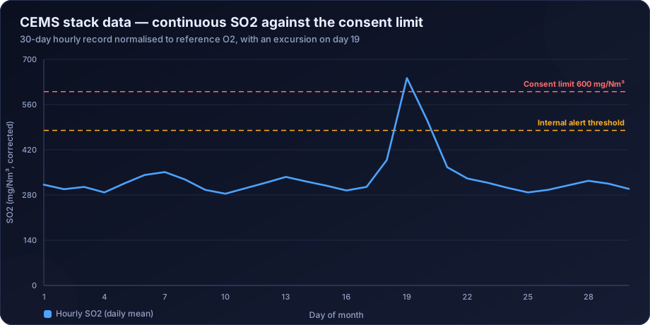
In the chart above, the day-19 excursion is a single sharp event reaching 642 mg/Nm³ against a 600 limit, with elevated values on either side. That shape — a build-up, a peak, a decay — points to a control device problem rather than an instantaneous process trip, and the operational log should say which.

Startup and shutdown periods are excluded from compliance assessment in many regimes, but only if properly defined, documented and flagged in advance. Retrospectively reclassifying an excursion as a startup is the kind of thing audits are designed to catch.

Statistical presentation

• Time series against the limit, with the limit line drawn
• Distribution and percentiles of the averaging-period values
• Cumulative frequency, showing what fraction of time is spent in each concentration band
• Excursion register with cause codes
• Availability statistics by month
• Correlation with production or load, normalised as emission per unit output

From Concentration to Emission Rate

Compliance is about concentration; inventories, dispersion modelling and carbon accounting need mass emission rate.

Emission rate (kg/h) = Concentration (mg/Nm³) × Flow rate (Nm³/h) × 10⁻⁶

Both terms must be on the same basis — dry, standard conditions, and if the concentration is oxygen-corrected the flow must correspond.

Flow measurement is often the weakest link. A 15% error in stack flow becomes a 15% error in emission rate, which propagates directly into every dispersion model result. Flow monitors should be verified against pitot traverse, and where CEMS flow is unavailable, flow is calculated from fuel consumption and stoichiometry — usually more reliable than a poorly maintained flow monitor.

Emission factors are derived by normalising emission rate to activity: kg per tonne of product, kg per tonne of fuel, g per kWh. These are what feed the emission inventory for dispersion modelling, and site-specific measured factors are always preferable to generic published values.

Linking Stack Data to Ambient Impact

Stack data is the input to the dispersion models that predict ground-level concentrations:

• Emission rate per source, at the correct averaging period
• Stack height, internal diameter, exit gas temperature and exit velocity
• Operating profile — hourly emission variation matters as much as annual total

Modelling with an annual-average emission rate under worst-case meteorology understates the peak; modelling with peak emissions under all meteorology overstates the annual mean. Serious assessments use an hourly emission file matched to the hourly meteorology, an approach covered in air dispersion modelling for EIA in India.

Stack data also supports stack height determination under CPCB guidance, where the required height is a function of emission rate — see stack height calculation under CPCB guidelines.

Common Errors in Stack Data Analysis

• Omitting the oxygen correction, or applying the wrong reference value for the source type
• Mixing wet and dry basis between measurement and limit
• Not normalising to standard temperature and pressure
• Comparing an hourly value against a 30-day rolling limit or vice versa
• Including calibration and maintenance periods in compliance statistics
• Unverified flow measurement propagating into every emission rate
• Ignoring the RATA result and continuing to report data from a CEMS that failed it
• Non-isokinetic manual sampling accepted because the laboratory result looked reasonable
• Computing availability over calendar hours rather than operating hours
• Reclassifying excursions as startup after the fact

How DSTechnoverse Helps

DSTechnoverse analyses source emission data for industries, consultancies and EPC contractors across India.

• CEMS data validation — status flag handling, drift and calibration review, RATA and CGA outcome integration, availability computation over operating hours, and full flagging with an audit trail.
• Correction and normalisation — standard conditions, moisture basis and reference oxygen applied correctly and documented, so every reported number is auditable against its consent condition.
• Compliance analysis — statistics computed at every relevant averaging period, excursion registers with duration, magnitude and cause classification, and trend analysis on excursion frequency as an early warning of equipment degradation.
• Emission rate and factor derivation — mass emission rates with verified flow, and site-specific emission factors normalised to production for inventory use.
• Dispersion model input preparation — hourly emission files, stack parameters and operating profiles prepared for AERMOD and CALPUFF modelling.
• Reporting — consent compliance reports, CEMS periodic returns, and emission inventory submissions structured to SPCB and CPCB expectations.

Where a facility is facing a compliance question, we analyse the source data and the surrounding ambient data together, because the two lines of evidence resolve disputes that neither settles alone.

---

Need air quality data turned into a defensible answer? DSTechnoverse provides end-to-end air quality analysis services — monitoring data validation, statistical analysis, source apportionment, dispersion modelling, GIS mapping, and regulator-ready reporting. Talk to our air quality team about your dataset or project.

Frequently Asked Questions

What is CEMS in air quality monitoring?

A Continuous Emission Monitoring System measures pollutant concentrations in flue gas continuously at the source, typically using extractive or in-situ analysers for SO2, NOx, CO, particulate matter and oxygen, together with flow and temperature. In India, CEMS installation with data transmission to regulators is mandatory for defined categories of highly polluting industries.

Why is oxygen correction applied to stack emission data?

Because diluting flue gas with excess air reduces the measured concentration without reducing the mass of pollutant emitted. Correcting to a reference oxygen level — commonly 6% for coal boilers and 3% for oil and gas — removes that loophole so the reported figure reflects actual emission rather than dilution.

What is isokinetic sampling and why does it matter?

Isokinetic sampling draws the sample at exactly the velocity of the flue gas at the sampling point. If the sampling rate is too low, heavier particles are over-collected; too high, and they are under-collected. An isokinetic ratio outside about 90–110% invalidates the particulate result regardless of laboratory quality.

What is a RATA test?

A Relative Accuracy Test Audit compares CEMS readings against simultaneous manual reference-method sampling, usually annually. It is the traceability anchor for the whole CEMS dataset — without a passed RATA, the continuous readings have no verified accuracy, however stable they appear.

What CEMS data availability is required?

Most regimes require 85–90% valid data during operating hours annually. Availability is computed over operating hours, not calendar hours, and missing periods are typically substituted with conservative high values so that downtime carries a compliance penalty rather than an advantage.

How is a mass emission rate calculated from a stack concentration?

Multiply the concentration in mg/Nm³ by the volumetric flow rate in Nm³/h and convert units, ensuring both are on the same temperature, pressure and moisture basis. Flow measurement accuracy is usually the limiting factor, so flow monitors should be verified against pitot traverse or cross-checked against fuel consumption.

Can stack monitoring data replace ambient monitoring?

No. Stack data quantifies what a source emits; ambient data measures what is in the air people breathe, which includes all other sources and the effects of dispersion. Compliance frameworks require both, and dispersion modelling is what links one to the other.

What is the difference between a wet and dry basis measurement?

A wet-basis concentration includes water vapour in the flue gas; a dry-basis concentration excludes it. Since flue gas moisture is commonly 8–20%, comparing a wet-basis measurement against a dry-basis limit understates the emission by that proportion. Every reported value must state its basis.