PM2.5 and PM10 Data Analysis: From Raw Monitor Output to Defensible Insight

Particulate matter is where most air quality analysis begins and where most of it goes wrong. PM data looks deceptively simple — one number, one unit, one standard — which encourages teams to average it, chart it, and declare a conclusion. In reality PM datasets carry a specific statistical shape, a set of internal consistency rules, a strong meteorological dependence, and a diagnostic structure that a competent analyst can read like a source inventory. This guide covers the full analytical treatment of PM2.5 and PM10 data, from the first validation check to the interpretation that goes into a report.

PM2.5 and PM10 data analysis is the process of validating particulate matter measurements, characterising their statistical distribution, computing compliance statistics against the applicable standard, decomposing variation into diurnal, weekly and seasonal components, and using derived metrics such as the PM2.5/PM10 ratio to attribute the measured burden to dust, combustion or secondary aerosol sources.

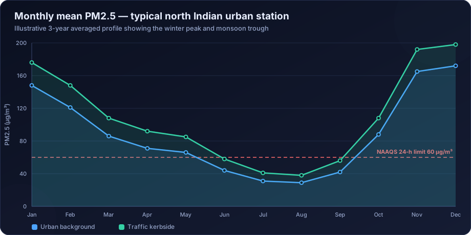
Start With What PM Data Actually Is

PM10 and PM2.5 are mass concentrations of particles below a size cut, in micrograms per cubic metre. Three properties follow, and each has analytical consequences.

PM2.5 is a subset of PM10. Physically, PM2.5 ≤ PM10 always. Any record violating this is invalid — not interesting, invalid. It usually indicates an instrument fault, a flow-rate error, a filter handling problem, or a channel mix-up in the data logger.

Concentrations are strongly right-skewed. The distribution is approximately log-normal: many moderate days, a long tail of severe episodes. This means the arithmetic mean sits above the median and is heavily influenced by a handful of episode days. Reporting only the mean is a defensible summary of total exposure but a poor description of a typical day. Report the median, the geometric mean and the percentiles alongside it.

Concentration reflects dilution as much as emission. Ambient PM is emission divided by the available mixing volume. A winter night with a 150 m inversion produces triple the concentration of a summer afternoon from identical emissions. Any analysis that reads a seasonal PM curve as an emissions curve is misreading it.

Step 1 — Validation Rules Specific to PM

Generic QA/QC applies (see QA/QC for air quality monitoring data), but PM has its own checks.

Check	Rule	Typical cause of failure
Size consistency	PM2.5 ≤ PM10 in every record	Channel swap, calibration drift, inlet blockage
Ratio plausibility	0.15 ≤ PM2.5/PM10 ≤ 0.95	Instrument fault, one channel offline
Negative values	Reject or flag; small negatives near zero may be instrument noise	Baseline drift on BAM/TEOM
Stuck values	Identical value repeated for many hours	Logger fault, frozen sensor
Rate of change	Implausible step change between consecutive hours	Power event, maintenance not flagged
Flow rate	Within manufacturer tolerance of the design flow	Pump degradation, filter loading
Filter handling (gravimetric)	Conditioning time, temperature and humidity within spec	Laboratory procedure deviation
Field blank	Blank mass below the method detection limit	Contamination during handling
Data capture	≥ 75% valid hours before publishing an average	Downtime, calibration, power

The flow rate check deserves emphasis. Gravimetric PM concentration is collected mass divided by sampled volume, and sampled volume is flow rate multiplied by time. A 10% flow error becomes a 10% concentration error that no downstream statistic can detect or correct.

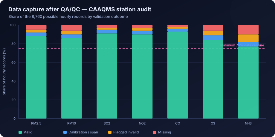
Step 2 — Describe the Distribution Correctly

Before any test, characterise the shape:

• Median and geometric mean describe the typical day.
• Arithmetic mean describes total mass burden and is what annual standards use.
• Percentiles (50th, 75th, 90th, 95th, 98th, 99th) describe the tail, which is where health impact and compliance failures concentrate.
• Maximum and the date it occurred — always report the date, because it is usually diagnostic (Diwali, a stubble-burning window, a dust storm, a plant upset).
• Coefficient of variation indicates whether the station is episode-driven or steadily loaded.

A box plot across stations is the fastest way to see structure that a table of means hides.

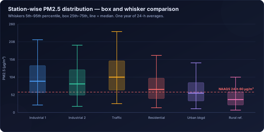
In the plot above, the traffic station has both the highest median and the widest spread, while the rural reference station is low and tight. The gap between the rural reference and the urban background is the regional background contribution; the gap between urban background and traffic is the local increment. That decomposition — available from nothing more than well-sited monitors and a box plot — is one of the most useful outputs in the whole discipline.

Step 3 — The PM2.5/PM10 Ratio as a Source Diagnostic

The ratio of fine to coarse particulate is a free source-apportionment signal available from any station measuring both.

Ratio	Interpretation	Typical setting
0.15–0.30	Strongly dust-dominated	Mining, quarrying, unpaved roads, arid pre-monsoon
0.30–0.45	Dust-dominated with combustion contribution	Construction-heavy urban, industrial estates
0.45–0.60	Mixed urban	Typical Indian city, annual average
0.60–0.75	Combustion-dominated	Urban winter, dense traffic, biomass use
> 0.75	Secondary aerosol dominated	North Indian winter smog episodes

Track the ratio month by month. A ratio that rises through October and November while absolute concentrations rise tells you the winter increment is combustion and secondary aerosol, not dust — which means road-sweeping and water-spraying will not fix it, and combustion controls will. A ratio that stays low while concentrations rise points to dust and a completely different control set.

The ratio is also a validation tool. A step change in the ratio with no corresponding change in either raw channel almost always indicates an instrument problem rather than an atmospheric one.

Step 4 — Exceedance and Compliance Statistics

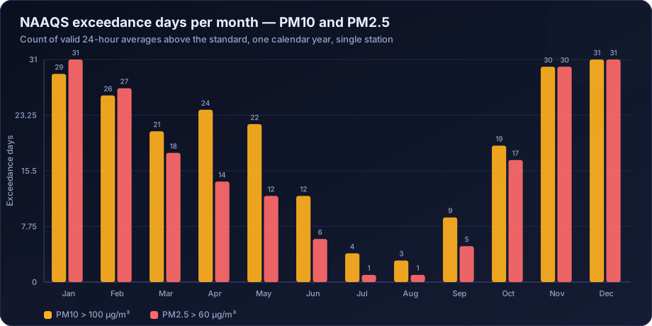
India's 24-hour standards (100 µg/m³ PM10, 60 µg/m³ PM2.5), notified by the Central Pollution Control Board, are 98th-percentile standards: exceedance is permitted on up to 2% of monitored days in a year, but not on two consecutive days. Compliance analysis therefore requires four numbers, not one:

1. Annual arithmetic mean versus the annual standard (60 PM10, 40 PM2.5).
2. Count of exceedance days and that count as a percentage of valid days.
3. The 98th percentile value of the ranked 24-hour series.
4. The longest run of consecutive exceedance days.

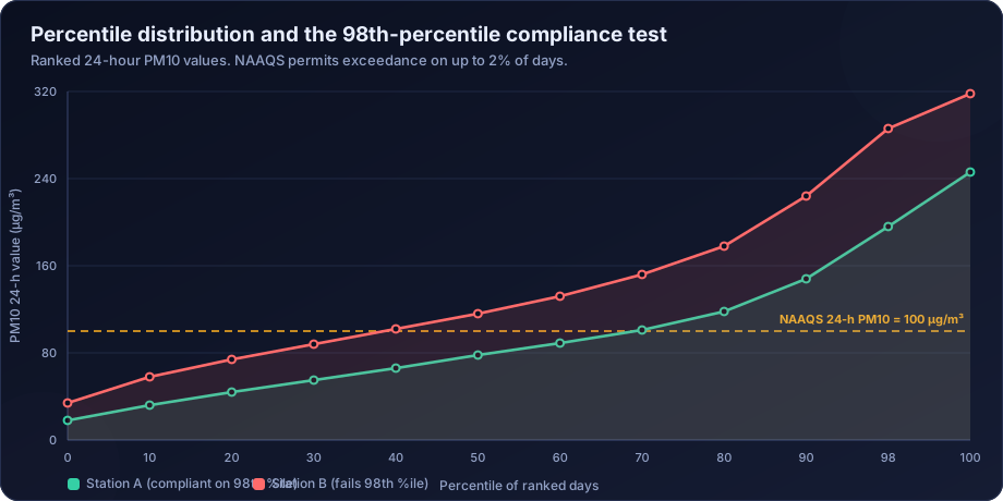
The chart makes the test concrete. Station A's 98th-percentile value sits below the standard even though it has some exceedance days — it passes. Station B's 98th percentile is far above — it fails, and the annual mean confirms it. Reporting only "number of exceedance days" without the percentile test is incomplete, and reporting only the annual mean hides episodic risk entirely.

Monthly exceedance counts show where the problem concentrates in time:

Step 5 — Decompose the Variation

PM concentration varies on four timescales, and separating them is the core analytical move.

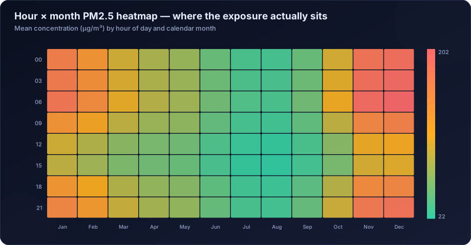
Diurnal (hour of day). Look for the pre-dawn maximum caused by boundary-layer collapse and the mid-afternoon minimum caused by maximum mixing depth. Twin traffic peaks superimpose on this. A station whose diurnal profile has no afternoon minimum is either affected by a continuous local source or has an instrument issue.

Weekly. A weekday–weekend difference is a traffic and industrial-activity signature. Its absence in a station you assumed was traffic-dominated is informative.

Seasonal. In most of India the pattern is a winter maximum, a sharp monsoon minimum from washout and deep mixing, and a pre-monsoon dust signal in the coarse fraction. Regional variations matter — coastal stations show a much flatter seasonal curve than the Indo-Gangetic Plain.

Episodic. Stubble burning windows, festival days, dust storms, plant upsets. These should be identified and reported separately, never quietly averaged in.

The hour-by-month heatmap collapses two of these dimensions into one readable figure:

Step 6 — Bring in Meteorology

PM analysis without meteorology is incomplete. The essential joins are:

• PM versus wind direction — a polar plot immediately reveals directional sources. If concentrations spike consistently from 240–270°, there is something to the west-southwest.
• PM versus wind speed — a concentration that falls with wind speed indicates a local ground-level source being diluted; a concentration that rises with wind speed indicates either resuspension or an elevated plume being brought down.
• PM versus mixing height — usually the dominant explanatory variable for seasonal variation.
• PM versus rainfall — washout, and the reason monsoon data must never be pooled with dry-season data in a single summary statistic.

This analysis is what separates "concentrations were high in December" from "concentrations were high in December because a 180 m nocturnal mixing height concentrated an emission load that was itself 20% higher due to biomass heating". Only the second statement supports a decision. See meteorological normalisation of air quality data.

Step 7 — Handle Gaps Honestly

Every real PM dataset has gaps. The analytical question is not how to fill them but whether to.

Gap length	Recommended treatment
1–2 hours	Linear interpolation acceptable, flag it
3–12 hours	Diurnal climatology or nearby-station regression, flagged
12–48 hours	Only with a validated co-located or nearby reference; document fully
> 48 hours	Leave as missing; adjust the data-capture statement

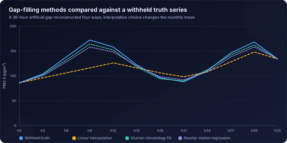
The comparison above is instructive: linear interpolation across a 36-hour gap that contained an episode flattens the peak entirely and biases the monthly mean low. A diurnal-climatology fill recovers the shape far better. Whichever method is used, filled values must be flagged in the delivered dataset, and any statistic computed from them must say so. Silently filled data that later appears in a regulatory submission is the kind of thing that ends careers.

Step 8 — Trend Analysis

Do not fit an ordinary least-squares line to PM data and report the slope — the openair package implements the correct alternative directly. The residuals are non-normal, autocorrelated and heteroscedastic, which invalidates the p-value. Use the non-parametric Mann–Kendall test for significance and the Theil–Sen estimator for slope, and normalise for meteorology before claiming a policy effect.

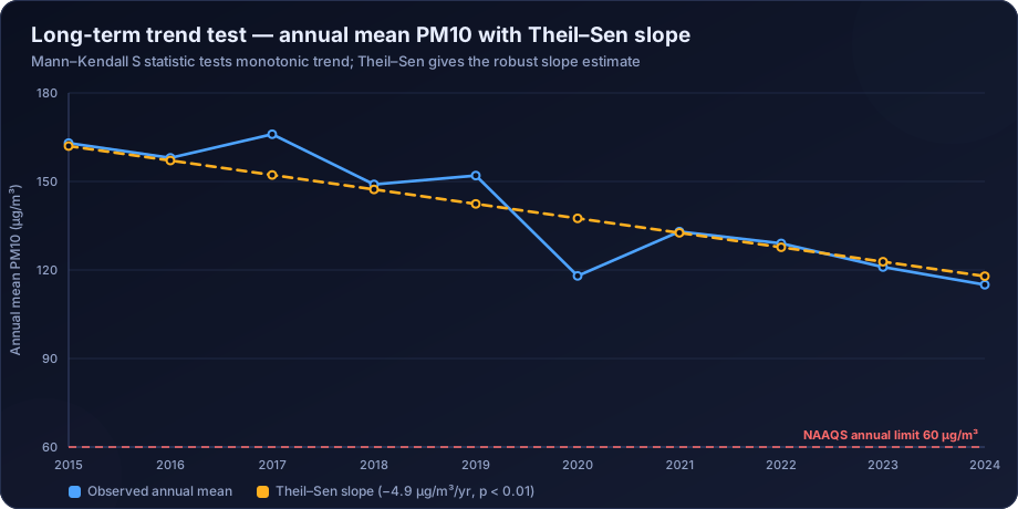
Full method treatment is in air quality trend analysis methods.

Interpretation Errors That Get Reports Rejected

• Reporting an annual mean from a single season. Non-monsoon-only monitoring produces a number well above the true annual mean. It is a valid seasonal statistic; it is not an annual one.
• Averaging across stations of different land-use classes and calling the result "the city's PM2.5".
• Comparing a 24-hour maximum against the annual standard, or vice versa.
• Presenting exceedance counts without the percentile test, or the percentile test without the consecutive-day rule.
• Ignoring the PM2.5 ≤ PM10 violation and averaging it in anyway.
• Attributing a fall in concentration to an intervention without meteorological normalisation, when the intervention year happened to be windy and wet.
• Using low-cost sensor PM data uncorrected, which typically over-reads by 20–60% at high relative humidity.
• Failing to state data capture, so the reviewer cannot judge how much weight any average deserves.

How DSTechnoverse Helps

DSTechnoverse runs particulate matter data analysis as a specialist service for consultancies, industries, municipal programmes and research groups.

What the engagement looks like. You send raw data in whatever form it exists — CAAQMS CSV exports, manual monitoring sheets, laboratory gravimetric results, sensor logs, or a mix. We audit it first and tell you honestly what it can and cannot support. We then run a scripted validation and analysis pipeline, and deliver both the outputs and the code.

What we analyse.

• Full PM-specific validation including size consistency, flow, ratio plausibility and blank correction
• Distribution characterisation with medians, geometric means and the full percentile suite
• 98th-percentile compliance testing, exceedance counts and consecutive-day runs against NAAQS
• PM2.5/PM10 ratio analysis as a source diagnostic, tracked seasonally
• Diurnal, weekly, seasonal and episodic decomposition
• Meteorological joins — polar plots, wind-speed dependence, mixing-height correlation
• Mann–Kendall and Theil–Sen trend testing with meteorological normalisation
• Documented, flagged gap treatment with a stated data-capture position

What you receive. A validated and versioned dataset, a statistical annexure, publication-quality figures, NAAQS comparison tables, an interpretation narrative, and a limitations statement — plus the R or Python scripts, so your team can rerun the analysis when next year's data arrives.

Where the project also needs predictive work, we connect the measured baseline to AERMOD dispersion modelling so incremental impact is assessed on the same basis as the measured background.

---

Need air quality data turned into a defensible answer? DSTechnoverse provides end-to-end air quality analysis services — monitoring data validation, statistical analysis, source apportionment, dispersion modelling, GIS mapping, and regulator-ready reporting. Talk to our air quality team about your dataset or project.

Frequently Asked Questions

What does the PM2.5/PM10 ratio tell you?

It indicates the balance between combustion-derived fine particles and mechanically generated coarse dust. A low ratio around 0.2–0.4 points to dust from roads, construction or soil; a high ratio above 0.7 points to combustion and secondary aerosol. Tracking the ratio seasonally shows whether the control strategy should target dust or combustion.

Why is PM data log-normally distributed and why does it matter?

Because concentration results from multiplicative processes — emission rate divided by a highly variable dilution volume. The consequence is a long right tail: the arithmetic mean is pulled well above the median by a few episode days. Summarising with the mean alone misrepresents typical conditions, so medians, geometric means and percentiles should be reported alongside.

How many days of data are needed for a valid PM analysis?

For comparison against a 24-hour standard, enough valid days to characterise the distribution and support a 98th-percentile test — practically a full season at minimum. For an annual mean, a full calendar year with at least 75% data capture. Short campaigns support screening statements only.

Can PM2.5 ever be higher than PM10 in valid data?

No. PM2.5 is physically a subset of PM10, so any record where PM2.5 exceeds PM10 indicates an instrument, calibration or data-handling error. Such records must be flagged and investigated, never averaged into a reported statistic.

What is the 98th percentile rule in Indian PM standards?

The 24-hour NAAQS limits may be exceeded on up to 2% of the monitored days in a year, but not on two consecutive days. Compliance assessment therefore requires ranking the 24-hour values, checking the 98th-percentile value against the limit, and separately checking for consecutive-day exceedances.

How should missing PM data be handled?

Short gaps of one or two hours can be linearly interpolated with a flag. Longer gaps are better filled using diurnal climatology or regression against a nearby station, and gaps beyond about two days should be left missing with the data-capture statement adjusted. Every filled value must be flagged in the delivered dataset.

Do low-cost sensors give usable PM2.5 data?

They give usable relative and spatial information after correction, but raw output is not comparable to reference data. Optical sensors respond to particle scattering, which varies with humidity and size distribution, and typically over-read substantially in humid conditions. Co-location with a reference monitor and a humidity-aware calibration are essential before the data is reported.

What is the difference between an exceedance day and non-compliance?

An exceedance day is any day whose 24-hour average is above the limit. Non-compliance is a legal determination that also considers the 98th-percentile test and the consecutive-day rule. A station can record several exceedance days and still comply; a station can record fewer and fail if they fall on consecutive days or push the 98th percentile above the limit.