Quick answer: Road and highway projects in India are modelled in AERMOD by converting traffic counts, vehicle mix and India-specific emission factors into an emission rate per metre of road, then representing each carriageway as RLINE, line, area or a string of volume sources. Receptors are placed in lines parallel to the corridor and at sensitive locations, and predicted increments of PM10, PM2.5, NO2 and CO are added to baseline values and compared with NAAQS 2009. Construction-phase dust from earthworks, batching and hot mix plants is assessed separately.
Highways, expressways, ring roads, flyovers and urban corridors change air quality in a way that industrial projects do not. The emission is spread along kilometres rather than released from a single stack, it is close to the ground, it peaks during commuting hours, and people live, study and trade within metres of the kerb. A credible air quality assessment for a road project therefore needs a different set of inputs and a different receptor design from a typical factory model.
This guide sets out when a road project needs dispersion modelling in India, how traffic emissions are estimated, how the road is represented in AERMOD (including the RLINE source types), how receptors should be laid out, and what to do about construction-phase dust. It ends with a worked example for a 10 km four-lane highway section, mitigation options and the mistakes that most often draw comments from reviewers.
When Road Projects Need Air Quality Modelling
Several situations lead to an air quality prediction for a road project.
- Environmental Clearance under the EIA Notification 2006. Highways appear as a separate item in the Schedule. Coverage depends on factors such as whether the road is a national or state highway, the length of new alignment or expansion, the additional right of way, and whether it passes through hilly terrain or ecologically sensitive areas. The thresholds have been amended more than once, so the current Schedule and any later notifications should be checked for each project. Where EC is needed, the Terms of Reference usually ask for baseline ambient monitoring, prediction of air quality impacts during construction and operation, and an environmental management plan.
- Multilateral and lender requirements. Projects financed by development banks often need an air quality assessment under the lender's environmental and social standards, even where Indian EC is not triggered.
- Urban corridors and flyovers. Elevated roads, grade separators and bus rapid transit corridors in dense cities may not need EC but are frequently assessed because of nearby schools, hospitals and housing.
- Projects next to a highway. A township, hospital or school planned beside an expressway may need near-road modelling to understand exposure, even though the road is not the project.
- Cumulative studies. Industrial parks and logistics hubs generate heavy goods traffic. Including the access road as a source makes the cumulative picture realistic; see our article on cumulative air quality impact assessment in India.
For the overall EIA process and where modelling sits within it, read our guide on air dispersion modelling for EIA in India.
Pollutants That Matter Near Roads
Road traffic emits NOx (mostly as NO, with a share of direct NO2), CO, PM from exhaust, PM from brake and tyre wear, resuspended road dust, hydrocarbons including benzene, and smaller amounts of other species. For an Indian road EIA, the pollutants usually modelled and compared with NAAQS 2009 are:
| Pollutant | NAAQS 2009 limits (µg/m³ unless stated) | Why it matters near roads |
|---|---|---|
| PM10 | 100 (24-h), 60 (annual) | Resuspended dust, brake and tyre wear, exhaust |
| PM2.5 | 60 (24-h), 40 (annual) | Diesel exhaust from trucks and buses; most closely linked to health effects |
| NO2 | 80 (24-h), 40 (annual) | Heavy vehicle exhaust; strong gradient within the first 100 to 200 m |
| CO | 4 mg/m³ (1-h), 2 mg/m³ (8-h) | Congested traffic, junctions and tunnels |
| Benzene | 5 (annual) | Petrol vehicles and evaporative losses, relevant near fuel stations and congested junctions |
24-hourly and 8-hourly values should be met 98% of the time in a year, with no exceedance on two consecutive days. Baseline values in many Indian corridors, particularly for PM10 and PM2.5, are already high, so the incremental contribution of the road and its share of the total are central to the assessment. Our explainer on NAAQS standards in India covers averaging periods and compliance in more detail.
Estimating Traffic Emissions
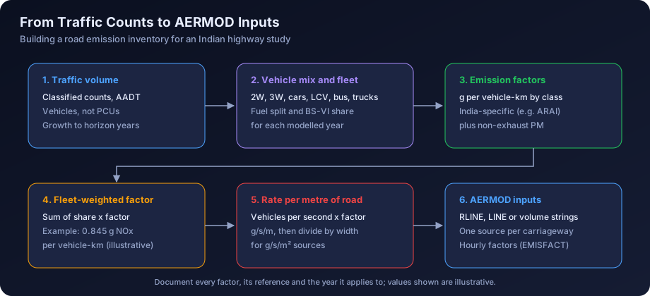
The emission inventory is where road studies most often fall short. AERMOD needs an emission rate, and for roads that rate is built from four inputs: traffic volume, vehicle mix, speed and emission factors.
Step 1: Traffic Volume
Use classified traffic volume counts from the project's traffic study, usually reported as annual average daily traffic (AADT) and as passenger car units. For modelling you need actual vehicle numbers by class, not passenger car units, because emission factors apply per vehicle. Projected traffic for the design horizon years comes from the traffic study's growth rates. Model at least the opening year and one or two horizon years, because the fleet mix and volume both change.
Step 2: Vehicle Mix
Split traffic into classes that match the available emission factors: two-wheelers, three-wheelers, cars (petrol, diesel, CNG), light commercial vehicles, buses, two-axle trucks and multi-axle trucks. On many national highways, heavy goods vehicles are a minority of the vehicle count but the majority of NOx and exhaust PM.
Step 3: Diurnal And Directional Pattern
Hourly counts show the daily cycle. Most Indian highways show morning and evening peaks for passenger vehicles and a night-time peak for trucks, partly because of city entry restrictions. Directional splits matter for divided carriageways modelled as separate sources. These patterns become hourly emission factors in AERMOD.
Step 4: Emission Factors
India-specific emission factors for vehicles were developed by the Automotive Research Association of India (ARAI) for CPCB, giving grams per kilometre by vehicle class, fuel, engine size and emission standard (Bharat Stage) era. Those factors are widely used in Indian EIAs and source apportionment studies. Some studies use international models adapted to Indian conditions. Whatever the source, document the factor, its reference and the vehicle class it applies to.
The move to Bharat Stage VI emission norms nationwide in April 2020 substantially tightened limits for new vehicles, particularly for NOx and PM from diesel vehicles. The on-road fleet changes gradually as older vehicles retire, so a sensible approach is to estimate the share of BS-VI vehicles in each class for each modelled year, using vehicle registration data or reasonable fleet turnover assumptions, and weight the emission factors accordingly. Avoid applying BS-VI factors to the entire fleet in the opening year: that understates emissions.
Step 5: Non-Exhaust PM
Brake wear, tyre wear and resuspended road dust can exceed exhaust PM on Indian roads, especially where shoulders are unpaved or silt loading is high. Methods such as the paved road equation in US EPA AP-42 estimate resuspension from silt loading and vehicle weight. Include it for PM10, and include the fine fraction for PM2.5.
Step 6: Convert To AERMOD Units
Combine the above into grams per vehicle kilometre for the fleet, multiply by vehicles per second, and you have grams per second per metre of road. For area-type sources, divide again by the width of the carriageway to get g/s/m². Our guide on emission inventories for dispersion modelling covers documentation of factors and assumptions.
Representing A Road In AERMOD
There are four common ways to put a road into AERMOD. Each has a place.
| Representation | AERMOD keyword | Emission rate unit | Strengths | Limitations |
|---|---|---|---|---|
| Roadway line source | RLINE | g/s/m² of road surface | Built for near-road dispersion; efficient for long corridors; handles road segments directly | Needs a recent AERMOD version; check which options remain beta in your release |
| Extended roadway source | RLINEXT | Per unit length of road (confirm in the User's Guide for your version) | Adds barriers, depressed roadways and elevation at each end | Some features remain non-regulatory; more inputs to justify |
| Line or area | LINE, AREA, AREAPOLY | g/s/m² | Familiar, widely accepted, handles receptors at the road edge | Slower for long corridors; less tailored to vehicle-induced turbulence |
| String of volumes | VOLUME | g/s per volume | Accepted method; same approach as haul roads | Exclusion zones near each volume; many sources for a long road |
RLINE And RLINEXT
The RLINE source type in AERMOD is derived from the R-LINE research model developed for near-road dispersion. It integrates emissions along the road segment numerically and includes treatment of vehicle-induced turbulence and the meandering of near-surface plumes in low wind. It entered AERMOD as an alpha and then beta option, and in recent AERMOD versions it has been promoted into the regulatory model, consistent with US EPA's latest revisions to its Guideline on Air Quality Models. RLINEXT is the extended form, with optional noise barriers and depressed roadway configurations and a separate elevation for each segment end.
Points to observe when using them:
- Check the AERMOD version and its model change bulletin to see which RLINE and RLINEXT features run under regulatory defaults and which need the BETA or ALPHA flags.
- Define each carriageway as a separate source, with its own width and traffic, so directional splits and the median gap are represented.
- Break the corridor into straight segments that follow the alignment. Curved sections need shorter segments.
- Use the initial vertical dimension to reflect vehicle wake mixing, with a documented basis.
- For flyovers, the deck height becomes the release height, and the ground below receives a lower near-road concentration than an at-grade road.
Line, Area And Volume Alternatives
Older and many current Indian studies use LINE or AREA sources for each carriageway, or a string of volumes. These remain acceptable when documented. Volume strings work well for short access roads. For volume sources, a common basis is a release height around half the top of the vehicle wake, an initial sigma-z of the wake height divided by 2.15, and an initial sigma-y of the volume spacing divided by 2.15, similar to the approach for haul roads.
Meteorology And Urban Settings
Road studies need the same hourly AERMET meteorology as industrial projects, and the same care over the source of surface and upper air data; see our guide on meteorological data for air modelling in India. For corridors through large cities, consider AERMOD's urban option with an appropriate population, because night-time urban heat island effects change dispersion compared with rural settings.
Receptors Along The Corridor
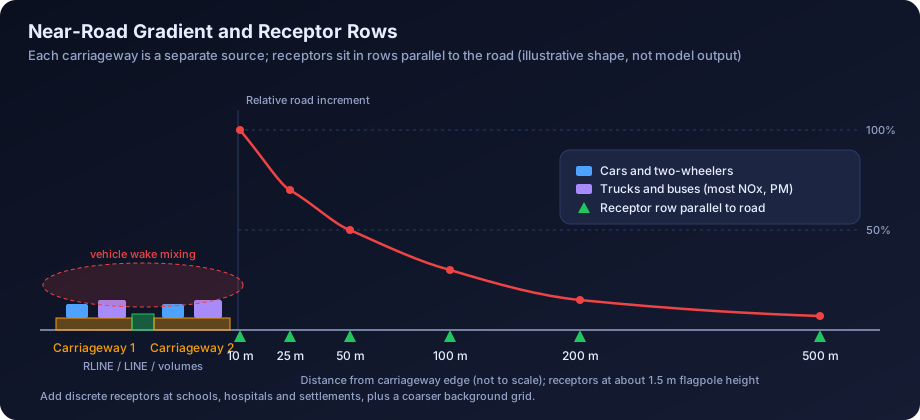
Receptor design has more effect on a road study than on most industrial studies, because the concentration gradient is steep. Concentrations of primary traffic pollutants generally fall sharply within the first 100 to 200 m of a busy road.
- Parallel receptor rows at set distances from the carriageway edge on both sides: for example 10, 25, 50, 100, 200 and 500 m.
- Spacing along the road of 100 to 250 m in typical sections, tighter at junctions, toll plazas and interchanges where traffic slows and queues.
- Discrete sensitive receptors at schools, hospitals, residential clusters, places of worship and markets, located from a current satellite image or survey.
- Breathing height. Use flagpole receptors at about 1.5 m for pedestrian exposure, and higher flagpoles for multi-storey buildings facing an elevated road.
- Background grid at coarser spacing to show the wider footprint.
Receptors placed on the carriageway itself are generally not meaningful for ambient air standards. Read our article on receptor grid design for dispersion modelling for more on nested grids and discrete receptors.
Near-Road PM2.5 And NO2
Two pollutants deserve particular care.
PM2.5. Diesel exhaust and fine resuspended dust are the main traffic contributions. Background PM2.5 in many Indian cities and the Indo-Gangetic Plain is often close to or above the NAAQS, so the road increment is usually small in proportion but still important for exposure. Report the increment, the baseline, the total and the share attributable to the road at each sensitive receptor.
NO2. Vehicles emit NOx mostly as NO, which converts to NO2 by reacting with ozone. Modelling all NOx as NO2 is conservative and often overstates near-road NO2. AERMOD offers conversion methods, including the Ambient Ratio Method 2 (ARM2), the Ozone Limiting Method (OLM), the Plume Volume Molar Ratio Method (PVMRM) and the Generic Reaction Set Method (GRSM). Methods that use ozone need hourly or representative background ozone data and an in-stack (here tailpipe) NO2 to NOx ratio, which is higher for modern diesel vehicles with oxidation catalysts than for older petrol vehicles. Document the ratio and the background ozone used. In AERMOD these options are set in the control pathway (for example the OLM or GRSM keyword with the NO2STACK and OZONEVAL or OZONEFIL inputs).
Construction-Phase Dust
Road construction often produces higher short-term dust than the operating road, and Terms of Reference usually ask for it. Typical sources are:
| Construction activity | Usual representation | Notes |
|---|---|---|
| Earthworks, cutting and filling along the alignment | Area or volume sources per active stretch | Model only the stretches active at one time |
| Borrow areas and quarries | Area or OPENPIT plus haul roads | Often outside the right of way; check locations |
| Hot mix plant | Point source for the stack, volume for aggregate handling | Plant-specific stack height and controls |
| Wet mix macadam and concrete batching plants | Volume sources | Cement silos as point sources if vented |
| Stone crushers | Volume sources | Use crusher and screen emission factors with controls |
| Unpaved haul and access roads | Volume strings | Watering frequency affects the control efficiency |
Construction modelling is normally presented as a reasonable worst case for a representative construction camp and active stretch, not the full corridor at once. Pair the results with a dust management plan: water sprinkling, covered transport, wheel washing, wind barriers and locating plants away from settlements. For guidance on how fugitive sources are typically treated, see our page on air quality modelling for mining projects, which uses similar methods.
Worked Example: A 10 km Four-Lane Highway Section
All numbers in this example are illustrative. They show the method and do not represent any real road, emission factor set or monitoring result.
Inputs
- Length: 10 km, at grade, four lanes divided (two carriageways of 7.0 m each, with a median)
- Traffic in the design year: 40,000 vehicles per day, split equally by direction
- Vehicle mix by count: cars 45%, two-wheelers 20%, light commercial 10%, buses 5%, trucks 20%
- Illustrative fleet-average emission factors in g/vehicle-km, already weighted for an assumed BS-VI share:
| Vehicle class | Share | NOx | PM2.5 exhaust |
|---|---|---|---|
| Cars | 45% | 0.10 | 0.005 |
| Two-wheelers | 20% | 0.10 | 0.010 |
| Light commercial | 10% | 0.30 | 0.030 |
| Buses | 5% | 3.0 | 0.10 |
| Trucks | 20% | 3.0 | 0.15 |
Step 1: Fleet-Weighted Factor
- NOx: 0.45 × 0.10 + 0.20 × 0.10 + 0.10 × 0.30 + 0.05 × 3.0 + 0.20 × 3.0 = 0.845 g/vehicle-km
- PM2.5 exhaust: 0.45 × 0.005 + 0.20 × 0.010 + 0.10 × 0.030 + 0.05 × 0.10 + 0.20 × 0.15 ≈ 0.042 g/vehicle-km
- PM10 including non-exhaust and resuspension: assume an illustrative 0.15 g/vehicle-km
Note how buses and trucks, 25% of vehicles, contribute about 89% of the NOx. That is why heavy vehicle numbers in the traffic study deserve close checking.
Step 2: Emission Per Metre Of Road
- NOx, both directions: 40,000 vehicles × 0.845 g/km = 33,800 g per km per day, which is 33.8 g per metre per day
- 33.8 ÷ 86,400 s ≈ 3.9 × 10⁻⁴ g/s per metre (daily average)
- Whole 10 km section: about 338 kg of NOx per day, or 3.9 g/s on average
- PM2.5 exhaust: 40,000 × 0.042 = 1,690 g/km/day, about 2.0 × 10⁻⁵ g/s per metre
- PM10 total: 40,000 × 0.15 = 6,000 g/km/day, about 6.9 × 10⁻⁵ g/s per metre
Step 3: Split Into Carriageways
- Each carriageway carries half: NOx about 1.96 × 10⁻⁴ g/s per metre
- For RLINE, LINE or AREA sources, divide by the 7.0 m carriageway width: 1.96 × 10⁻⁴ ÷ 7.0 ≈ 2.8 × 10⁻⁵ g/s/m²
- Segment each carriageway to follow the alignment, for example 20 straight segments of about 500 m each
Step 4: Hourly Profile
From the hourly traffic counts, derive 24 hourly factors that average to 1.0. In this illustration, cars and two-wheelers peak at 9 to 10 am and 6 to 8 pm, and trucks peak between 10 pm and 4 am. Because trucks dominate NOx, the NOx profile peaks at night, when the atmosphere is stable and dispersion is weakest. This is one reason near-road NO2 can be higher at night than the daytime traffic count suggests. The factors are applied with the EMISFACT keyword using HROFDY, or with separate factors for weekdays and weekends if counts show a difference.
Step 5: Receptors
- Receptor rows at 10, 25, 50, 100, 200 and 500 m from each carriageway edge, every 200 m along the road, at 1.5 m flagpole height
- Discrete receptors at an illustrative school 60 m from the edge and a village cluster 150 m from the edge
- A coarser background grid out to about 2 km
Step 6: Run, Convert And Combine
- Run NOx with a documented NO2 conversion method using background ozone
- Run PM10 and PM2.5 as separate pollutants
- Add predicted 24-hour and annual increments to baseline monitoring values at each receptor
- Present the highest values, the values at sensitive receptors, and the share from the road
Step 7: Present The Gradient
A table such as the one below, filled with model results, helps reviewers and the public see the near-road pattern. The values here are relative and illustrative only, to show the typical shape, not a model output.
| Distance from carriageway edge | Relative road increment (illustrative) |
|---|---|
| 10 m | 100% |
| 25 m | about 70% |
| 50 m | about 50% |
| 100 m | about 30% |
| 200 m | about 15% |
| 500 m | under 10% |
The actual gradient depends on meteorology, road height, barriers, terrain and the receptor height. Our guide on reading AERMOD output and contour maps explains how to present corridor contours clearly.
Mitigation For Road Projects
Mitigation should follow from the results, particularly where sensitive receptors lie close to the alignment.
- Alignment and setback. Shifting the alignment, adding a bypass, or keeping new schools and hospitals back from the edge is the most effective long-term measure.
- Vegetation barriers. Dense, multi-row green belts with suitable species can reduce near-road concentrations behind them when designed properly; gaps and sparse planting have little effect.
- Solid barriers and noise walls. These alter near-road dispersion and can be represented with RLINEXT options; document whether you used them in regulatory runs.
- Traffic management. Smoother flow at toll plazas (electronic tolling), junction design and reduced idling cut CO and NOx at hot spots.
- Paved shoulders and road cleaning. Reduce silt loading and resuspended dust.
- Construction dust controls. Sprinkling, covered trucks, wheel washing, enclosed batching and setback of hot mix plants and crushers from settlements.
Common Mistakes In Road AERMOD Studies
- Using passenger car units instead of vehicle counts when applying emission factors.
- Ignoring non-exhaust PM, which can dominate PM10 on Indian roads.
- Applying BS-VI factors to the whole fleet in the opening year.
- Flat 24-hour emissions that ignore night-time truck peaks.
- All NOx treated as NO2 without saying so, or a conversion method used without documenting background ozone and tailpipe NO2 ratios.
- Too few receptors near the road, so the steepest part of the gradient is missed.
- Volume sources with receptors inside exclusion zones, returning zeros at the road edge.
- One source for both carriageways on a wide divided road, losing directional and median effects.
- Using an AERMOD version where RLINE is still beta without stating it, or assuming every RLINEXT feature is regulatory.
- Construction modelled for the whole corridor at once, which overstates impacts, or not at all, which leaves a ToR item unanswered.
Our broader list of common AERMOD mistakes applies to road studies too. If you are deciding whether AERMOD is the right tool or a dedicated line source model would suit better, see our AERMOD versus CALPUFF and model selection guide.
How DSTechnoverse Helps
DSTechnoverse builds air quality assessments for highway, expressway, flyover and urban corridor projects, from traffic-based emission inventories and fleet assumptions to RLINE, line or volume source setups, near-road receptor design, NO2 conversion and construction-phase dust modelling. Our AERMOD modelling service supports Environmental Clearance and lender studies, including white-label work for EIA consultancies. Road source types are handled by our modelling team, while AERMOD Studio covers point-source runs such as hot mix plant stacks. To scope your corridor study, talk to our team.
Regional guides: for local regulators, industrial areas and meteorological data in fast-growing corridors, see AERMOD modelling in Delhi NCR, Mumbai, Pune and Maharashtra and Bengaluru and Karnataka.
Frequently Asked Questions
Do highway projects in India need air dispersion modelling? Highway projects that need Environmental Clearance under the EIA Notification 2006 usually receive Terms of Reference asking for prediction of air quality impacts during construction and operation, which in practice means dispersion modelling. Coverage depends on the type of highway, length, right of way and terrain, and the thresholds have been amended, so check the current Schedule for each project.
What is RLINE in AERMOD? RLINE is a roadway source type in AERMOD derived from the R-LINE research model, designed for near-road dispersion of traffic emissions. It integrates emissions along road segments and accounts for near-surface plume behaviour. It has been promoted into the regulatory model in recent AERMOD versions. RLINEXT extends it with barriers and depressed roadways, though some features may still require non-default flags.
How are traffic emissions calculated for AERMOD? Start with classified vehicle counts and projections, split traffic by vehicle class and fuel, apply emission factors in grams per vehicle kilometre, and weight them by fleet share. Multiply by vehicles per second to get grams per second per metre of road, then divide by carriageway width for area-type sources. Hourly profiles from traffic counts are applied as emission factors.
Which emission factors are used for Indian vehicles? Indian studies commonly use emission factors developed by ARAI for CPCB, which give grams per kilometre by vehicle class, fuel and emission standard era. Some studies use international models adapted to Indian fleets. The factors should be weighted for the expected share of BS-VI vehicles in each modelled year, and the source of every factor should be cited in the report.
How far from a highway should receptors be placed? Place receptor rows parallel to the carriageway at close distances, such as 10, 25, 50, 100, 200 and 500 metres from the edge, because concentrations fall steeply within the first 100 to 200 metres. Add discrete receptors at schools, hospitals and settlements, use about 1.5 metre flagpole height for breathing level, and include a coarser background grid.
How is NO2 modelled near roads? Vehicles emit NOx mostly as NO, which converts to NO2 by reacting with ozone. Treating all NOx as NO2 is conservative. AERMOD offers ARM2, OLM, PVMRM and GRSM conversion methods. Ozone-based methods need background ozone data and a tailpipe NO2 to NOx ratio, both of which should be documented and justified in the report.
Should construction dust be modelled for road projects? Yes, where the Terms of Reference ask for construction-phase impacts, which is common. Model representative active stretches, borrow areas, hot mix plants, batching plants, crushers and haul roads rather than the whole corridor at once. Combine the results with a dust management plan covering sprinkling, covered transport, wheel washing and siting of plants away from settlements.
Can AERMOD Studio model a highway? AERMOD Studio currently models point sources on flat terrain with regulatory defaults, so it suits stacks such as hot mix plant or DG set stacks associated with a road project. Road corridors modelled with RLINE, line, area or volume sources are set up and run by the DSTechnoverse modelling team, who can integrate both sets of results.
Does a flyover change air quality predictions compared with an at-grade road? Yes. An elevated deck raises the release height, which generally lowers concentrations at ground level directly beneath and close to the structure, while upper floors of buildings facing the deck may receive higher exposure. Model the deck height as the release height, and use elevated flagpole receptors for buildings at deck level.
Need an AERMOD study or AERMOD software? DSTechnoverse runs regulatory AERMOD modelling studies for EC, CTE and expansion applications, for industries and as a white-label partner for EIA consultancies, and provides AERMOD Studio, our AERMOD software, personalised for your firm. We are based in Indore, Madhya Pradesh and work across India. Talk to our team.