Every air quality conclusion rests on an assumption that is almost never stated: that the numbers are real. Instruments drift, pumps degrade, loggers freeze, calibrations lapse, power fails mid-average, and analysts paste columns into the wrong place. Quality assurance and quality control is the discipline that turns a raw data stream into a dataset you can defend in front of a regulator, a reviewer, or a court. It is unglamorous, it is where most of the hours go on a serious project, and it is the first thing a competent auditor examines.
This guide sets out the full QA/QC procedure for ambient air quality monitoring data: the difference between QA and QC, the instrument-side controls, the data-side validation tests, flagging conventions, calibration traceability, gap treatment, the data capture rule, and the documentation that makes the whole thing auditable.
QA/QC for air quality monitoring data is the combined set of preventive procedures (quality assurance — siting, calibration schedules, standard operating procedures, training) and corrective checks (quality control — range tests, consistency tests, drift analysis, flagging) applied to raw measurements to produce a validated dataset with a documented data-capture rate, a complete audit trail, and a stated uncertainty.
QA and QC Are Not the Same Thing
The terms are used interchangeably and they should not be.
Quality assurance is preventive and happens before and during measurement. It covers station siting, instrument selection and certification, calibration schedules, standard operating procedures, operator training, chain of custody for filters, and the design of the monitoring programme itself. QA determines the ceiling on data quality — no amount of post-processing will rescue a monitor sited two metres from an idling truck bay.
Quality control is corrective and happens to the data. It covers validation tests, flagging, drift correction, gap treatment and the completeness assessment. QC determines how much of the theoretically achievable quality you actually retain.
A project with excellent QC and poor QA produces a beautifully validated record of the wrong thing.
Part 1 — Quality Assurance: Getting It Right Before the Data Exists
Station siting
Siting errors are unrecoverable. The core requirements:
- Inlet height typically 3–10 m above ground, and consistent across a network so stations are comparable.
- Clear sky angle — no obstruction within a specified arc; a general rule is that the distance to any obstacle should be at least twice the height by which it exceeds the inlet.
- Distance from roads appropriate to the station's purpose. A kerbside station is meant to be near traffic; an urban background station is not, and siting it near a bus stand invalidates its classification.
- Distance from local interferences — DG sets, kitchens, parking areas, waste burning, air-conditioning exhausts.
- Representativeness — the station must represent the land-use class it is assigned to, because that classification determines which standard applies and how the data is interpreted.
- Security and power stability, because the largest single cause of data loss in Indian networks is power interruption.
Instrument selection and certification
Use reference or reference-equivalent methods where the endpoint is compliance. The designated methods and their performance specifications are documented by the US EPA Ambient Monitoring Technology Information Center and, for India, in the CPCB monitoring guidelines published at cpcb.nic.in. For PM this means gravimetric or a certified BAM; for gases, the designated analyser principle — UV fluorescence for SO2, chemiluminescence for NOx, NDIR for CO, UV photometry for O3. Certification status should be documented in the report, not assumed.
Calibration regime
| Activity | Typical frequency | Purpose |
|---|---|---|
| Zero and span check | Daily (automatic) | Detect drift early |
| Multipoint calibration | Monthly or quarterly | Verify linearity across the range |
| Flow rate verification | Monthly | Ensure sampled volume is correct |
| Leak check | Monthly | Detect dilution of the sample |
| Converter efficiency (NOx) | Quarterly | Verify NO2 to NO conversion |
| Performance audit (independent) | Annually | External verification against traceable standards |
| Microbalance calibration (gravimetric) | Per weighing session | Mass traceability |
Every calibration standard must be traceable to a recognised reference. A span gas cylinder without a valid certificate makes every measurement it calibrated unverifiable.
Standard operating procedures and training
Written SOPs for sampling, filter handling, data download, and incident recording, with operators trained against them. Filter handling in particular is where gravimetric datasets are lost: conditioning time, temperature and humidity control in the weighing room, static control, handling with forceps only, and field blanks carried through the whole process.
Part 2 — Quality Control: Validating the Data
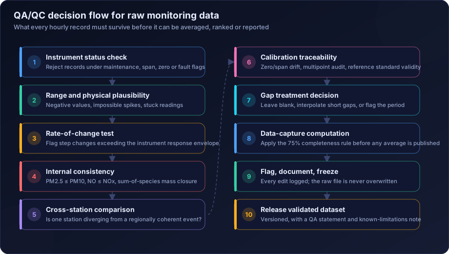
The validation sequence below is applied in order, because later tests assume earlier ones have passed.
Test 1 — Instrument status and operational flags
Reject or flag any record recorded during maintenance, calibration, span, zero, fault or power-restoration periods. Automatic analysers write these flags themselves; the frequent failure is that the export ignores the flag column and the calibration spikes enter the dataset as real measurements. A characteristic signature is an implausibly clean square-wave pattern in a concentration series at a fixed time each day — that is the daily span check being reported as ambient air.
Test 2 — Range and physical plausibility
Each parameter has a physically possible range and an instrument-specific measurement range. Values outside either are invalid. Small negative values near zero are normal instrument noise on some analysers and are usually retained (or set to half the detection limit) with a flag; large negatives are faults.
Test 3 — Rate-of-change test
Compare consecutive values against the maximum plausible change given the instrument's response time and realistic atmospheric variability. A jump from 40 to 900 µg/m³ in one hour is either a genuine, explainable event (a dust storm, a nearby fire) or a fault — and the analyst's job is to determine which, not to delete it silently.
Test 4 — Stuck-value and flatline detection
Identical values repeated over many consecutive intervals almost always indicate a frozen logger or a failed sensor rather than genuinely constant air. Set a threshold appropriate to the parameter's normal variability.
Test 5 — Internal consistency
| Consistency rule | Why |
|---|---|
| PM2.5 ≤ PM10 | Physical subset relationship |
| NO ≤ NOx and NO2 = NOx − NO | Definitional |
| Sum of speciated mass ≤ total PM mass | Mass closure |
| AQI sub-index ≤ 500 | Scale bound |
| Relative humidity 0–100% | Physical bound |
| Wind direction 0–360° | Physical bound |
| Calm-wind flag consistent with wind speed threshold | Sensor stall detection |
The wind sensor stall check is worth calling out. Cup anemometers and vanes have a starting threshold; below it they report a fixed direction and zero speed. A dataset where wind direction sits at exactly the same value for hours at low speed is recording a stalled sensor, not a persistent breeze, and any polar plot built on it is fiction.
Test 6 — Cross-station and cross-parameter coherence
Regional pollution episodes are spatially coherent. If five stations in a city rise together and one falls, the one is suspect. Conversely, if one station spikes alone, it may be a genuine local source — which is a finding, provided you have checked the alternative.
Cross-parameter coherence is equally useful: a genuine combustion event raises PM2.5, CO and NOx together. A PM2.5 spike with no corresponding CO or NOx response is more likely dust, a filter artefact, or an instrument problem.
Test 7 — Drift analysis
Plot zero and span check results over time. A slowly rising zero indicates baseline drift that has been quietly inflating every measurement since the last calibration. Where drift is detected, the affected period may be correctable by linear back-adjustment between calibration points — but the correction must be documented and the corrected values flagged.
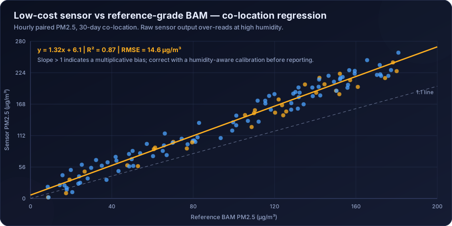
Test 8 — Comparison against co-located or reference instruments
Where a reference instrument is co-located, regression of the field instrument against it gives slope, intercept and R². This is the standard approach for low-cost sensor calibration and is equally applicable to verifying a continuous analyser against gravimetric reference samples.
Flagging: The Convention That Makes Everything Traceable
Never delete data. Flag it. A deleted record cannot be reviewed, reversed or explained; a flagged record can.
A workable flag scheme:
| Flag | Meaning | Use in statistics |
|---|---|---|
| V | Valid | Include |
| C | Calibration / span / zero period | Exclude |
| M | Maintenance | Exclude |
| F | Failed a validation test | Exclude |
| S | Suspect — retained pending review | Exclude by default, document |
| B | Below detection limit | Include, substituted per policy |
| I | Interpolated / gap-filled | Include only with disclosure |
| A | Adjusted for drift | Include, adjustment documented |
| N | No data — instrument offline | Exclude, counts against capture |
Two rules make the scheme work. The raw file is never modified. All flags and adjustments live in a working copy with a change log. And every statistic reports the flags underlying it, so a reader can see that a monthly mean was built from 612 V records and 48 I records rather than 660 unqualified numbers.
Gap Treatment
Gaps are inevitable. Filling them is a decision with consequences, and the decision must be explicit.
| Gap length | Default treatment | Notes |
|---|---|---|
| 1–2 hours | Linear interpolation, flagged I | Low risk |
| 3–12 hours | Diurnal climatology or nearby-station regression, flagged I | Preserves shape better than linear |
| 12–48 hours | Only with a validated predictor; otherwise leave missing | Document the method and its error |
| > 48 hours | Leave missing | Adjust data capture; do not fabricate |
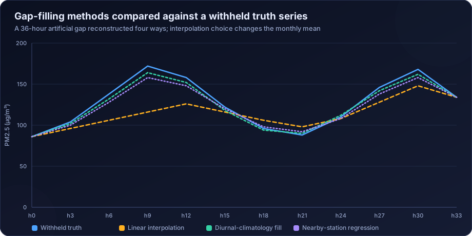
The figure shows why method choice matters. A 36-hour gap that happened to contain an episode is flattened by linear interpolation, which biases both the monthly mean and — more seriously — the exceedance count downward. A diurnal-climatology or regression fill preserves the shape. Whichever is used, the honest position is to run the headline statistics both with and without filled values and report if the conclusion changes.
The Data Capture Rule
Data capture is the percentage of possible measurements that are valid after QC. It is the single most important number in a QA/QC statement, and it belongs in the report, not in an annexure.
The general rule: at least 75% valid data in an averaging period before a mean may be published. Applied at each level:
- 24-hour average — at least 18 valid hours (some programmes accept 16).
- Monthly average — at least 75% of valid days.
- Annual average — at least 75% of valid days, and many protocols additionally require reasonable distribution across seasons so a year is not built from one dry season.
- 8-hour rolling mean (O3, CO) — at least 6 valid hours in the window.
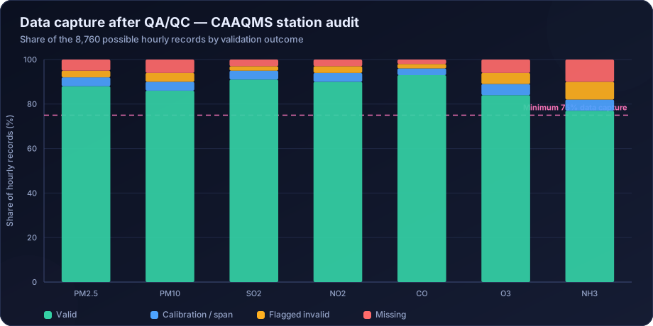
Distribution matters as much as the total. A year with 78% capture concentrated in the monsoon and post-monsoon, missing most of winter, satisfies the arithmetic test and fails the representativeness test badly. State the seasonal distribution of valid data explicitly.
Documentation: What an Auditable QA/QC Record Contains
- Station metadata: coordinates, land-use classification, inlet height, surroundings, photographs, commissioning date
- Instrument inventory: make, model, serial number, measurement principle, certification status
- Calibration log: dates, standards used, traceability certificates, pre- and post-adjustment values
- Maintenance log: every intervention with date, reason and effect on data
- Validation record: tests applied, thresholds used, records flagged and why
- Gap register: every gap with duration, cause and treatment
- Data capture statement: per parameter, per period, with seasonal distribution
- Version control: dataset version, date, author, and change log
- Known limitations: stated plainly
If a reviewer cannot reconstruct how a published number came from a raw measurement, the QA/QC record is inadequate regardless of how careful the work was.
Common QA/QC Failures in Practice
- Calibration periods left in the ambient dataset, creating recurring artificial spikes.
- Deleting rather than flagging, destroying the audit trail.
- Data capture never stated, so the reader cannot weight the conclusions.
- Wind sensor stall unnoticed, producing a wind rose that is an artefact.
- Filter blanks not run, so gravimetric results carry uncorrected handling contamination.
- Flow rate assumed rather than verified, producing a systematic concentration bias.
- Gap filling undocumented, so interpolated values become "measurements".
- Editing the raw file, after which nothing can be verified.
- Seasonal imbalance ignored, so an "annual" mean is really a dry-season mean.
- No independent audit, so systematic errors persist across years unchallenged.
How DSTechnoverse Helps
DSTechnoverse performs air quality data validation as a standalone service and as the mandatory first stage of every analysis project we take on. We do not analyse unvalidated data, because the analysis would be precise and meaningless.
Data validation and audit. We take raw exports from CAAQMS systems, manual monitoring programmes, sensor networks or laboratory records and run a scripted validation pipeline covering every test described above. You get back a flagged, versioned dataset, a validation report listing exactly what was found and what was done, and a data-capture statement per parameter and per period.
QA programme design. For clients establishing or expanding a network, we advise on station siting and classification, instrument selection, calibration schedules, SOP development and operator training, and we build the data pipeline so validation happens continuously rather than as a scramble before a submission.
Third-party QA/QC audit. Independent review of an existing dataset or monitoring programme, which is frequently commissioned before a regulatory submission, during due diligence, or when a dataset is being challenged. We have found calibration spikes in published data, stalled wind sensors driving three years of source attribution, and "annual" means built from seven months of one season.
Reporting. A QA/QC chapter written to withstand scrutiny, with methods, thresholds, flags, capture rates and limitations documented in full — the same standard we apply in EIA data analysis outsourcing and in dispersion modelling report QA.
Need air quality data turned into a defensible answer? DSTechnoverse provides end-to-end air quality analysis services — monitoring data validation, statistical analysis, source apportionment, dispersion modelling, GIS mapping, and regulator-ready reporting. Talk to our air quality team about your dataset or project.
Frequently Asked Questions
What is the difference between QA and QC in air quality monitoring?
Quality assurance is preventive and happens before and during measurement — siting, instrument certification, calibration schedules, SOPs and training. Quality control is corrective and happens to the data — range tests, consistency checks, drift analysis, flagging and gap treatment. QA sets the achievable quality ceiling; QC determines how much of it you keep.
What is the 75% data capture rule?
It requires that at least 75% of the possible measurements in an averaging period be valid before an average is published. In practice this means at least 18 valid hours for a 24-hour mean, and at least 75% of valid days for a monthly or annual mean. Averages computed from less data must be flagged as indicative rather than reported as compliant statistics.
Should invalid air quality data be deleted?
No. Invalid records should be flagged with a code indicating why they failed, and excluded from statistics — but retained in the dataset. Deleting data destroys the audit trail and makes the validation unreviewable. The raw file should never be modified at all; all flagging happens on a working copy with a change log.
How do you detect instrument drift?
By plotting the results of routine zero and span checks over time. A steadily rising zero indicates baseline drift inflating all measurements; a changing span response indicates sensitivity drift. Where drift is confirmed, values between calibration points can sometimes be corrected by linear back-adjustment, provided the correction is documented and the adjusted values flagged.
What are the most common air quality data errors?
Calibration and span periods left in the ambient dataset, unverified flow rates producing systematic bias, stalled wind sensors generating fictitious wind roses, undocumented gap filling, deleted rather than flagged records, and data capture that is never stated. Most of these are invisible in the final chart and obvious in the raw record.
How often should air quality analysers be calibrated?
Automatic zero and span checks should run daily, multipoint calibration monthly to quarterly depending on the instrument and programme, flow verification and leak checks monthly, NOx converter efficiency quarterly, and an independent performance audit annually against traceable standards.
Can gap-filled data be used in a regulatory submission?
Only if it is clearly flagged and the method documented. Short gaps filled by interpolation are generally accepted; long gaps filled by modelling are not a substitute for measurement. Best practice is to compute the headline statistics both with and without filled values and disclose whether the conclusion changes.
What should a data capture statement include?
The percentage of valid records per parameter and per averaging period, the seasonal distribution of those valid records, the causes of the largest gaps, and whether the capture meets the applicable rule. A single annual percentage without seasonal breakdown can hide a dataset that is arithmetically adequate and analytically unrepresentative.