
Air is not the only medium regulators care about. Any project that discharges treated effluent, cooling water, or brine into a river, lake, estuary, or sea has to show the receiving water will stay within safe limits. Water dispersion modelling is how that is demonstrated.
Two zones, two questions
Water dispersion modelling splits into two stages, each answering a different question.
Near-field: how fast does it mix?
Right at the outfall, the effluent jet mixes rapidly with the surrounding water through momentum and buoyancy. Near-field modelling (using tools in the CORMIX family, for example) predicts the initial dilution achieved within the regulatory mixing zone — the limited area where concentrations are allowed to exceed ambient standards before diluting.
The key output: does the plume dilute enough by the edge of the mixing zone to meet the standard?
Far-field: where does it go?
Beyond the mixing zone, ambient currents, tides, and river flow carry the diluted plume across the wider water body. Far-field modelling predicts how pollutants, nutrients, or heat spread over larger distances and longer times, and whether sensitive locations downstream stay protected.
What gets modelled
- Conventional pollutants and nutrients against water-quality criteria
- Thermal plumes from power plant and industrial cooling water
- Brine from desalination reject streams
- Dilution of STP and CETP discharges
The inputs it needs
- The discharge: flow rate, temperature, and pollutant concentrations
- The receiving water: bathymetry, currents, tides, or river-flow regime
- The outfall: location, depth, and diffuser configuration
- The standards: ambient water-quality criteria and mixing-zone rules
Why outfall design is part of the study
If the plume does not dilute enough, the answer is often engineering: move the outfall to deeper or faster-moving water, or add a multi-port diffuser to boost initial mixing. Good water dispersion modelling does not just assess a design — it helps shape one that passes.
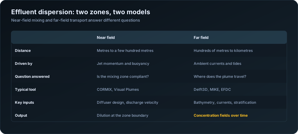
Two zones, two models, two questions
Effluent discharge is modelled in two stages because two different physical processes govern it, and one model cannot do both well.
| Near field | Far field | |
|---|---|---|
| Scale | Metres to a few hundred metres | Hundreds of metres to kilometres |
| Driven by | Discharge momentum and buoyancy | Ambient currents, tides, wind |
| Timescale | Seconds to minutes | Hours to days |
| Question answered | Is the mixing zone compliant? | Where does the plume travel? |
| Typical tools | CORMIX, Visual Plumes | Delft3D, MIKE, EFDC, Telemac |
| Key inputs | Diffuser design, exit velocity, density difference | Bathymetry, currents, stratification, tides |
| Output | Dilution achieved at a given distance | Concentration fields over space and time |
The near field is where the discharge's own energy dominates. A jet leaving a diffuser port entrains ambient water and dilutes rapidly — often achieving dilutions of 20 to 100 within tens of metres if the diffuser is well designed. The far field is where that initial energy is spent and the plume simply goes wherever the water goes.
Regulatory compliance is usually assessed at the edge of a defined mixing zone, which sits at the boundary between the two. Getting the near field right therefore determines whether the discharge complies; getting the far field right determines where the residual impact falls.
The inputs, and which ones actually matter
| Category | Parameters |
|---|---|
| Effluent | Flow rate, temperature, salinity or density, pollutant concentrations |
| Outfall | Depth, port diameter, number of ports, spacing, orientation, discharge angle |
| Receiving water | Depth, ambient current speed and direction, temperature and salinity profile |
| Dynamics | Tidal range and phase, seasonal flow variation, wind-driven circulation |
| Background | Existing concentrations of each modelled parameter |
| Standards | Discharge consent limits, receiving water quality criteria |
Density difference is the parameter that most changes behaviour and is most often supplied carelessly. Effluent warmer or fresher than the receiving water is buoyant and rises; cooler or more saline effluent sinks. A thermal discharge into the sea forms a surface plume; a brine discharge from a desalination plant forms a dense bottom current that behaves entirely differently and affects benthic habitat rather than surface waters.
Stratification is the other decisive input. A stratified water column can trap a rising plume beneath the thermocline, preventing it from reaching the surface and confining it to a layer where dilution is much slower. Modelling a stratified system as uniform substantially overstates dilution.
Outfall design is part of the study
Unlike air dispersion, where stack design is usually fixed before modelling, effluent modelling is frequently used to design the outfall. The parameters that matter:
| Design choice | Effect on dilution |
|---|---|
| Discharge depth | Deeper gives more water column for entrainment |
| Multi-port diffuser rather than single pipe | Dramatically better — often several times the dilution |
| Port diameter | Smaller ports give higher velocity and more entrainment |
| Port spacing | Too close and adjacent plumes merge, reducing dilution |
| Discharge angle | Typically 30 to 60 degrees upward for buoyant plumes |
| Orientation relative to current | Perpendicular to the prevailing current maximises mixing |
| Distance from shore | Further out generally means stronger ambient currents |
A multi-port diffuser is usually the single most cost-effective improvement available. Replacing an open-ended pipe with a diffuser of eight to twelve ports can raise near-field dilution by a factor of several, at a fraction of the cost of treating the effluent to a correspondingly lower concentration. Modelling several diffuser configurations before construction is therefore genuinely valuable engineering rather than a compliance exercise.
Scenarios that must be run
A single run at average conditions does not characterise a discharge. The critical case is a combination of conditions, and it is rarely the average.
| Scenario | Why |
|---|---|
| Maximum discharge, minimum ambient current | The worst dilution case |
| Slack tide | Near-zero current in tidal waters |
| Lean season river flow | Minimum dilution in freshwater discharges |
| Peak stratification | When trapping is most likely |
| Spring and neap tides | Different flushing behaviour |
| Seasonal current reversal | Where the plume direction changes |
| Plant upset or bypass conditions | Short-term elevated concentrations |
Slack tide is the case most often missed in coastal assessments. For an hour or so around high and low water, current speed approaches zero, and near-field dilution depends almost entirely on the discharge's own momentum. If a design relies on ambient current for dilution, its worst hour occurs twice a day, every day.
Where this fits in an EIA
| Assessment element | What the model supplies |
|---|---|
| Mixing zone compliance | Dilution and concentration at the zone boundary |
| Receiving water quality impact | Concentration fields across the study area |
| Thermal impact | Temperature rise contours, and delta-T at the boundary |
| Benthic impact | Bottom concentrations for dense discharges |
| Sensitive habitat exposure | Concentrations at mangroves, coral, spawning grounds |
| Water intake interaction | Whether the discharge recirculates to an intake |
| Cumulative assessment | Combined effect of multiple discharges |
The intake recirculation check deserves attention on any site with both an intake and an outfall. A discharge that returns to the plant's own intake raises intake temperature or salinity, degrades process efficiency and compounds over time. Modelling reveals it before construction, when the layout can still be changed.
The parallel with air, and where it breaks
Both disciplines model the transport of a release through a fluid, and both compare predicted concentrations against standards at defined receptors. The similarities in workflow — input assembly, scenario definition, standards comparison, QA of a traceable report — carry across directly, and the review discipline in how to QA/QC an air dispersion modelling report applies with little modification.
Where they differ: water bodies are bounded and their geometry dominates the result, so bathymetry matters far more than terrain does in air modelling. Tidal reversal means the receiving water moves back and forth over the same area, accumulating rather than dispersing in one direction. And density effects, which are minor in air dispersion beyond initial plume rise, govern the entire behaviour of an effluent plume.
For the air-side equivalents see AERMOD vs CALPUFF and how to prepare an emission inventory. Our water and effluent dispersion modelling service covers near-field and far-field studies for EIA and consent applications. Discharge standards are published by the Central Pollution Control Board.
The takeaway
Water dispersion modelling turns "the discharge should be fine" into a defensible, quantified case. For consultancies without in-house hydrodynamic modelling, it is a natural service to offer through a specialist partner.
Frequently Asked Questions
What is water dispersion modelling?
The simulation of how a discharge — treated effluent, cooling water, brine — mixes into and travels through a receiving water body. It is run in two stages: near-field mixing driven by the discharge's own momentum and buoyancy, and far-field transport driven by ambient currents.
What is the difference between near-field and far-field modelling?
Near-field covers the first metres to a few hundred metres, where the discharge's own momentum and buoyancy dominate mixing, and determines mixing zone compliance. Far-field covers hundreds of metres to kilometres, where ambient currents govern where the plume travels.
What is a mixing zone?
The defined area around an outfall within which water quality standards may be exceeded while initial dilution occurs. Compliance is assessed at its boundary, which is why near-field dilution modelling determines whether a discharge is acceptable.
Which model is used for effluent dispersion?
CORMIX and Visual Plumes for near-field mixing; Delft3D, MIKE, EFDC or Telemac for far-field transport. Most assessments use one of each, with near-field results providing the source condition for the far-field model.
Does outfall design affect dilution?
Substantially. Replacing an open-ended pipe with a multi-port diffuser can increase near-field dilution several times over, usually far more cheaply than treating the effluent to an equivalently lower concentration. This is why modelling should inform outfall design rather than follow it.
What is the worst-case scenario for an effluent discharge?
Maximum discharge flow combined with minimum ambient current — typically slack tide in coastal waters or lean-season flow in rivers — often with peak stratification. It is rarely the average condition, and a study run only at average conditions does not characterise the discharge.
Need a modelling or EIA data desk without the overhead? DSTechnoverse works as a confidential, white-label subcontractor for air and water dispersion modelling and EIA data analysis. Get in touch to scope your next project.