Microbiological Trend Analysis: Statistical Process Control for Count Data

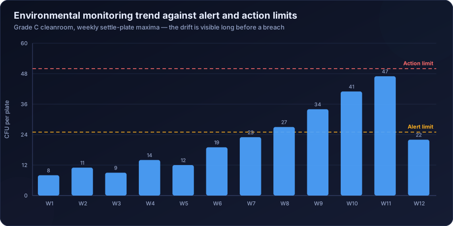
Most microbiological programmes generate far more information than they use. Results are compared against a limit, filed, and never looked at again — which means a process drifting steadily toward failure is invisible until the day it crosses. Trend analysis is what converts a compliance record into an early warning system, and it is the single highest-return improvement available to most testing programmes.

Why Pass or Fail Wastes the Data

A result of 400 CFU/g against a limit of 1000 is compliant. If every prior batch ran below 50, it is also the most important piece of information the laboratory produced that month.

Binary reporting cannot express that. It records a pass, the batch releases, and the signal is lost. Three months later the count crosses 1000, an OOS investigation begins, and the investigation discovers a trend that had been visible in the data for twelve weeks.

The chart above is a real pattern: a Grade C cleanroom where weekly settle plate counts climbed steadily from 8 to 47 across eleven weeks. Every single result was below the action limit of 50. A programme checking only limits saw eleven consecutive passes.

Microbiological Data Is Log-Normal

This is the technical point that most in-house trending gets wrong, and it invalidates the charts that follow from it.

Microbial counts are not normally distributed. They are approximately log-normal — bounded at zero, right-skewed, with occasional very high values. Applying standard normal-distribution control limits to raw counts produces two failures: a lower control limit that is negative and therefore meaningless, and an upper control limit that is too high, so genuine excursions do not trigger.

Transform the data before charting. Use log₁₀(count), or log₁₀(count + 1) to handle zeros. Calculate control limits on the transformed values, then back-transform for presentation if the audience prefers CFU. The mean of the log-transformed data corresponds to the geometric mean, which is the appropriate measure of central tendency for this kind of data.

Choosing the Right Chart

Data type	Chart	Notes
Counts per unit, moderate to high	Individuals and moving range on log₁₀	The general workhorse
Counts with many zeros	Positive-rate p-chart	Proportion of samples with any growth
Counts per defined area or volume	c-chart or u-chart	Poisson-based, suits low counts
Presence/absence	p-chart	Proportion positive over time
Multiple sites compared	Individual charts per site	Never aggregate across sites

That last row is the most commonly ignored. Charting the facility-wide average hides the one location that is deteriorating, because thirty-nine stable sites dilute it. Each site needs its own chart.

Positive Rate: The Better Metric in Clean Environments

In a well-controlled cleanroom, most results are zero. A chart of counts is then almost entirely flat at zero with occasional single-colony spikes, and conventional control limits are useless.

The more sensitive measure is the recovery rate — the percentage of samples showing any growth at all. A facility where 4 per cent of sites are positive is in a different state from one where 18 per cent are, even if every individual count is 1 or 2 CFU and every result is within limits.

This metric detects deterioration far earlier than magnitude does in low-bioburden environments, and it is the one we recommend as the primary trend indicator for Grade A and B monitoring.

Run Rules: Detecting Drift Before a Breach

A single point outside a control limit is the crudest signal. Run rules detect patterns that indicate a process shift while every individual point is still in range.

1. One point beyond three standard deviations — the classic out-of-control signal.
2. Two of three consecutive points beyond two standard deviations on the same side.
3. Four of five consecutive points beyond one standard deviation on the same side.
4. Seven or more consecutive points on the same side of the centre line — a sustained shift.
5. Seven or more consecutive points steadily increasing or decreasing — a trend.
6. Fifteen consecutive points within one standard deviation — unusually low variability, which often indicates data that is not what it appears to be.

Rule 6 deserves comment. Microbiological data is naturally variable. A long run of implausibly consistent results is worth investigating, and it occasionally reveals that testing was not actually performed as recorded.

Deriving Alert and Action Limits From Your Own Data

Copying limits from a guidance table is widespread and self-defeating. A Grade C action limit of 50 CFU per contact plate is meaningless in a facility that has never exceeded 8 — it will never trigger, and by the time it does the facility has deteriorated dramatically.

Limits should be statistical descriptions of your own performance, capped by any regulatory maximum.

• Alert limit — approximately the 95th percentile of routine historical data, or mean plus two standard deviations on log-transformed values.
• Action limit — approximately the 99th percentile, or mean plus three standard deviations, never exceeding the regulatory maximum.
• Minimum data set — at least 30 to 50 results per site before deriving limits, and preferably a full year to capture seasonality.
• Non-parametric methods where the zero fraction is high, since normal-distribution statistics fit badly.
• Annual review, plus review after any facility change, since limits derived three years ago describe a facility that no longer exists.

Seasonality Is Real and Should Not Be Treated as Drift

In Indian facilities, monsoon humidity and summer temperature produce predictable annual variation in microbiological counts. A programme that has not decomposed seasonality will interpret every June as an excursion and every January as an improvement.

Decompose the series into trend, seasonal and residual components. What matters is the trend after seasonal adjustment, and a rise that exceeds the seasonal expectation. A supplier or facility whose counts rise in step with the season is behaving normally; one whose counts rise outside that pattern warrants investigation.

Capability Analysis: How Much Margin Is There?

Control charts answer whether the process is stable. Capability analysis answers whether a stable process is good enough.

For microbiological data, calculate capability against the specification using log-transformed values. A process with a geometric mean of 50 CFU/g and a specification of 1000 has substantial margin. One with a mean of 400 against the same limit is stable but fragile — a modest shift produces failures.

This distinction matters commercially. Two products can both have a perfect release record while one is running at 5 per cent of its limit and the other at 40 per cent. The second will start failing, and capability analysis identifies it years before the first OOS.

Practical Implementation

1. Collect at least 30 to 50 historical results per site or product before deriving anything.
2. Log-transform, using log₁₀(count + 1) to accommodate zeros.
3. Chart individuals and moving range per site, never aggregated.
4. Track positive rate alongside magnitude in low-count environments.
5. Apply run rules, not just limit checks.
6. Derive alert and action limits from the distribution, capped at regulatory maxima.
7. Decompose seasonality before interpreting trend.
8. Calculate capability against the specification.
9. Review formally at a defined interval — monthly for environmental monitoring, quarterly for product release.
10. Document actions taken in response to signals, since an unactioned signal is worse than no signal at all.

What Trending Catches That Testing Does Not

• A water system developing biofilm, visible as a slow HPC rise months before coliforms appear.
• A cleaning procedure degrading as an operator's technique drifts, visible as a rising positive rate at specific sites.
• A supplier deteriorating, visible in incoming material counts before any lot fails.
• A preservative system weakening across a product's shelf life, visible in stability data before a challenge test fails.
• HVAC filtration losing performance, visible as rising mould recovery in specific areas.
• A new operator whose gowning technique is not yet reliable, visible in personnel monitoring by individual.

How DSTechnoverse Helps

Statistical trending is where our data analysis background matters most, and it is the layer most contract laboratories do not provide at all.

We deliver per-site and per-product control charting on correctly transformed data, positive-rate tracking for low-bioburden environments, run-rule based drift detection, alert and action limit derivation from your own historical data using methods appropriate to count distributions, seasonality decomposition, capability analysis against specification, and a monthly or quarterly review that says what the data means rather than restating it.

Clients frequently send us twelve months of results expecting confirmation that everything passed. The more useful output is usually the drift nobody had charted.

Common Trending Mistakes

• Charting raw counts instead of log-transformed values, which produces control limits that are mathematically wrong and practically useless.
• Aggregating sites or products, which hides the single deteriorating location behind the stable majority.
• Using guidance-table limits that are far above facility capability and therefore never trigger.
• Checking limits without run rules, so a sustained shift within limits goes unnoticed.
• Treating seasonality as drift, generating investigations every monsoon and false confidence every winter.
• Setting limits once at qualification and never revisiting them, so they describe a facility that has since changed.
• Excluding excursions from the limit calculation, which artificially tightens limits and produces constant false signals — or, done the other way, including a period of known contamination, which inflates limits so nothing ever triggers.
• Charting without acting. An unactioned signal is worse than no chart, because the record now shows the organisation saw the drift and did nothing.

That last point is the one with regulatory consequences. A trend chart in a file, with a clear eleven-week rise and no corresponding investigation record, is stronger evidence against a manufacturer than having no chart at all.

Frequently Asked Questions

Why log-transform microbiological data?

Because it is log-normally distributed. Applying normal-distribution control limits to raw counts gives a negative lower limit and an upper limit too high to trigger on genuine excursions.

How much data is needed before setting limits?

At least 30 to 50 results per site or product, and preferably a full year to capture seasonal variation. Limits derived from a handful of results will be wrong in both directions.

Should alert and action limits ever exceed the regulatory maximum?

No. Derive from your own data, then cap at the regulatory limit. Where your capability is better than the regulation, the tighter limit is the useful one.

What if most of our results are zero?

Chart the positive rate rather than the magnitude. In low-bioburden environments the proportion of sites showing any growth is far more sensitive than the count.

How often should trends be reviewed?

Monthly for environmental monitoring and water systems, quarterly for product release, and annually as a formal programme review that reassesses sites, limits and frequencies.

Can trending be done in a spreadsheet?

Yes, and for most facilities that is the right starting point. Log transformation, individuals charts and the standard run rules are all straightforward in Excel or Google Sheets. What matters is that the transformation is applied, the charts are per-site rather than aggregated, and someone reviews them on a defined schedule. Dedicated software helps at scale but is not the barrier — the barrier is almost always that nobody is charting at all.

What should a trend review actually produce?

A short written output stating what changed, what it probably means, and what will be done — not a pack of charts. The most common failure mode we see is a monthly trend report that reproduces the data faithfully and draws no conclusion. If the review does not end in either "no action, process stable" or a specific action with an owner, it has not been a review.

Does trending replace specification limits?

No, it complements them. The specification determines whether a batch releases. The trend determines whether the process is heading somewhere you do not want it to go.

---

Need release testing that produces insight rather than a pass or fail? DSTechnoverse provides finished product microbiological testing with statistical trending, objectionable organism assessment and OOS investigation support — from our Indore laboratory, for manufacturers across India. Talk to our microbiology team.