A four-year record shows no significant trend. Does that mean air quality is unchanged?
Almost certainly not. It means four years cannot detect the size of change that is plausibly occurring. Those are entirely different statements, and conflating them is one of the more consequential errors in air quality reporting — it can be read as evidence that an intervention failed when the data was never capable of showing success.
What Determines Detectability
Four factors, in roughly descending order of influence:
Trend size. By far the largest. Detecting a 5% annual decline is dramatically easier than detecting 1%.
Variability. The noisier the series, the longer the record needed. Urban sites with strong episodic behaviour are noisier than regional background sites.
Record length. Power increases with the number of periods, and roughly with the square of the span for trend detection — an extra few years at the end of a record is worth more than it looks.
Data capture. Gaps reduce effective sample size, and gaps clustered in one season do worse than that: they bias as well as weaken.
The interaction that matters: halving the trend you want to detect roughly quadruples the record needed. Small trends are disproportionately expensive to demonstrate.
Indicative Requirements
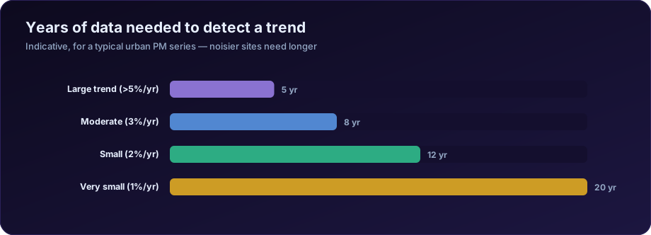
These are order-of-magnitude figures for a typical urban PM series with reasonable capture. Noisy sites need longer; clean regional sites less.
| Trend to detect | Indicative years needed |
|---|---|
| Large, above 5% per year | 5–6 |
| Moderate, around 3% per year | 8–10 |
| Small, around 2% per year | 12–15 |
| Very small, around 1% per year | 20+ |
Most real policy-driven changes fall in the 2–4% per year range, which is why eight to ten years is the usual practical minimum for a defensible trend statement, and why claims made on three or four years should be treated sceptically regardless of the p-value.
Why Short Records Mislead in Both Directions
False negatives. The common case. A genuine improvement exists but the record is too short to demonstrate it. Reported as "no significant trend", which readers hear as "no improvement".
False positives. Less common but more damaging. In a short noisy record, a couple of unusual years at either end can produce an apparently significant trend that is meteorological. A run of still winters at the start and windy ones at the end manufactures a decline.
The second failure is why endpoint sensitivity is worth checking directly: re-run the analysis dropping the first year, then the last year. If the conclusion changes, the record is too short to support it, whatever the test says.
Power Analysis Before You Start
The professional move is to ask, before analysing: given my record length and variability, what size of trend could I detect if it were there?
The approach:
- Estimate the year-to-year variability from your existing data
- Set the significance level and desired power, conventionally 0.05 and 80%
- Compute the minimum detectable trend for your record length
- Compare that against the change you are hoping to demonstrate
If the minimum detectable trend is 4% per year and the intervention plausibly delivers 2%, the analysis cannot succeed. Better to know that in advance than to report a null result that gets misread.
A useful reframing for reports: rather than "no significant trend", write "no trend detected; this record could detect a decline of 4% per year or larger". That is honest, informative, and cannot be misquoted as evidence of no change.
Getting More From a Short Record
Use monthly rather than annual values, with a seasonal test. More data points, more power — at the cost of handling autocorrelation. See the Mann-Kendall test.
Normalise for meteorology. Removing weather-driven variance reduces the noise the trend must overcome, and can meaningfully shorten the record needed. See meteorological normalisation.
Pool across stations. A regional trend across several sites has more power than any one site, if the sites genuinely share a regime.
Improve data capture. Filling gaps at the source is worth more than any statistical technique applied afterwards.
Use a precursor with a stronger signal. NO2 often responds to traffic measures more sharply than PM2.5, because PM has large regional and secondary components. A detectable NO2 change can evidence an intervention that PM cannot yet show.
Reporting an Inconclusive Result
An inconclusive result is a legitimate finding and should be written as one:
| Do | Do not |
|---|---|
| State the minimum detectable trend | Say "no change" |
| Give the slope with its interval | Report only the p-value |
| State the record length and capture | Leave the basis unstated |
| Say what would be needed to conclude | Imply the question is closed |
A worked example of good phrasing:
Over 2019–2025 the Theil-Sen slope was −1.2 µg/m³ per year (95% CI −3.4 to +0.9, p = 0.28), based on seven annual means with capture above 78%. The record is consistent with a decline of up to 3.4 µg/m³ per year but does not exclude no change. A record of this length and variability can reliably detect declines of approximately 3% per year or larger.
That paragraph cannot be misread. "No significant trend" can.
Designing a Network for Trend Detection
If the question is being asked before monitoring starts — or before a network is expanded — several design choices determine whether trends will ever be detectable.
Consistency beats sophistication. A modest instrument run identically for fifteen years produces better trend data than a superior instrument replaced twice. Every method change introduces a step that competes with the signal.
Siting stability matters more than siting perfection. A slightly compromised site kept constant is more useful for trends than an ideal site that moves. Relocation ends the record in practice.
Capture is worth more than resolution. Continuous monitoring at 90% capture beats higher-frequency monitoring at 60%, particularly if the missing 40% clusters seasonally.
Include a background or reference site. A regional reference station is what allows a local change to be distinguished from a regional one, and it is the single most valuable addition to a network for attribution purposes.
Record the metadata from day one. Instrument model, serial number, calibration history, siting details, and every change with its date. This costs almost nothing while the network runs and is irrecoverable afterwards. Most disputed long-term trends come down to metadata nobody kept.
Co-locate during any transition. Running the old and new instruments together for a few months quantifies the step, which allows the two periods to be joined into one usable record rather than two short ones.
Communicating Power to Decision Makers
The statistical point has to survive translation, because the audience for a trend analysis is usually not statistical.
Avoid the phrase "not significant" unedited. It is heard as "no effect". Pair it with the detectable size every time.
Use a measurement analogy. A useful one: measuring a change this small with this record is like weighing a letter on a bathroom scale — the letter has a weight, the instrument cannot resolve it, and that is a statement about the instrument rather than the letter.
Show the interval visually. A slope with its confidence band communicates uncertainty far better than a p-value in a table. Decision makers read the band correctly even when they would not interpret a p-value.
Say what would change the answer. "Three more years at current capture would allow a 2% per year decline to be detected" turns an inconclusive result into a plan rather than a dead end.
Separate the two questions explicitly. Whether air quality is improving, and whether this record can demonstrate it, are different. Reports that conflate them cause interventions to be judged on evidence that was never capable of assessing them.
Frequently Asked Questions
Can I claim a trend from three years of data? Only if it is very large and you state the caveats. Three years cannot support a policy conclusion about a modest change.
Does more frequent data compensate for a shorter record? Partly. Monthly values give more points than annual, but autocorrelation means the gain is less than the raw count suggests. Span matters more than frequency.
What if I have gaps? Reduced effective sample size and lower power. Gaps clustered by season also bias the result — report capture and its distribution.
Is 75% capture enough? It is the usual reporting threshold, not a guarantee of adequate power. Both matter separately.
How do I explain "no significant trend" to a non-technical audience? As "the data cannot yet distinguish a change of this size from normal year-to-year variation", with the detectable size stated.
Does meteorological normalisation really help? Yes, materially, by removing a large share of the variance the trend must exceed.
What is the single best way to improve future trend detection? Uninterrupted, well-calibrated monitoring with consistent methods. No analysis recovers what was never measured.
Need to prove an air quality change is real? DSTechnoverse runs trend analysis, meteorological normalisation and compliance reporting on monitoring data — with the uncertainty stated, not hidden. We are based in Indore, Madhya Pradesh and work with clients across India. See our air quality analysis service, or talk to our team.