
Ambient air quality data anchors the air-environment chapter of an EIA. It establishes what people are already breathing before a project starts, and it is the yardstick against which modelled impacts are judged. Analysing it well is a mix of careful statistics and correct standards.
The parameters that matter
Most ambient air quality campaigns monitor:
- Particulate matter — PM10 and PM2.5
- Gases — SO2, NOx (as NO2), CO, and often O3
- Site-specific pollutants — depending on the project (e.g. NH3, HC, heavy metals)
Each is measured over a monitoring period across several stations, usually covering different directions and land uses around the site.
Step 1: Validate the data
Before any statistic is computed, the dataset is screened for:
- Missing readings and data-capture rates
- Physically impossible values and outliers
- Consistent units and detection-limit handling
Step 2: Compute the required statistics
For each pollutant and station, the analysis reports minimum, maximum, mean (often the 98th percentile for short-term standards), and the number of exceedances. The averaging period must match the standard — 24-hour for PM, annual for long-term limits.
Step 3: Compare against NAAQS
Every result is placed against the National Ambient Air Quality Standards (or the applicable local/WHO limit). A clear comparison table shows whether the baseline is already near, at, or below the permissible level for each parameter.
Step 4: Visualise spatially and temporally
- Spatial maps show which parts of the study area are cleaner or more loaded
- Time-series plots reveal trends and episodic peaks
- Wind-linked analysis connects high readings to source directions
Step 5: Interpret for the assessment
The write-up explains what the baseline shows and, crucially, how much headroom exists below the standard — because that headroom is what a new source will consume.
Getting it right
Ambient air quality analysis is repetitive but unforgiving: a wrong averaging period or a misapplied standard can invalidate a conclusion. Standardised templates, correct statistics, and full traceability are what make the chapter defensible — and are exactly what a dedicated EIA data desk delivers consistently across projects.
The statistic that belongs against each standard
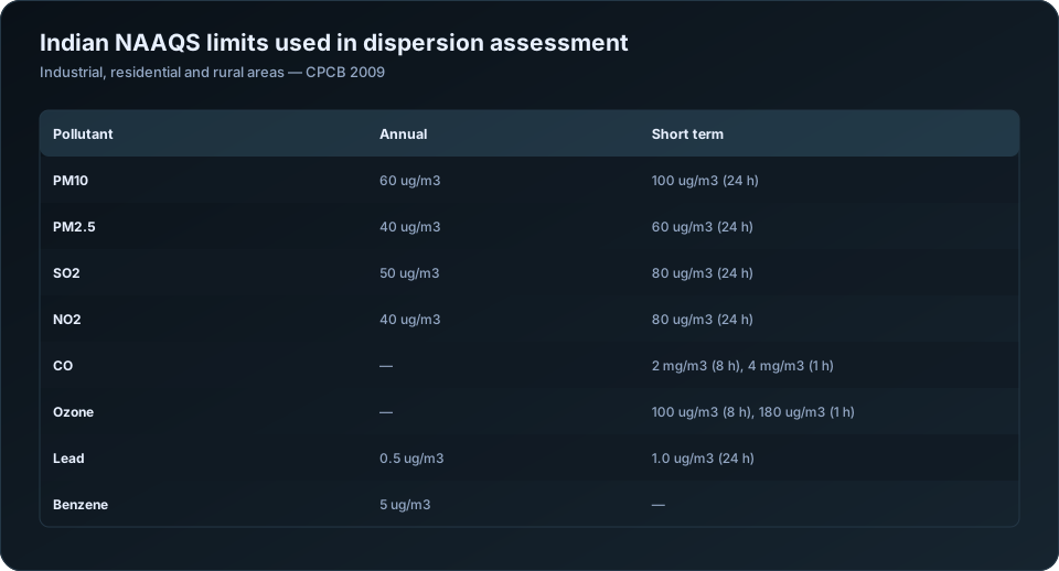
The most frequent defect in EIA air quality chapters is comparing the wrong number against the limit. Indian NAAQS defines short-term standards with a 2% exceedance allowance, which means the value to report is generally not the maximum.
| Pollutant | Averaging period | Limit (industrial, residential, rural) | Statistic to report |
|---|---|---|---|
| PM10 | Annual | 60 ug/m3 | Arithmetic mean |
| PM10 | 24-hour | 100 ug/m3 | 98th percentile of 24-hour values |
| PM2.5 | Annual | 40 ug/m3 | Arithmetic mean |
| PM2.5 | 24-hour | 60 ug/m3 | 98th percentile |
| SO2 | Annual | 50 ug/m3 | Arithmetic mean |
| SO2 | 24-hour | 80 ug/m3 | 98th percentile |
| NO2 | Annual | 40 ug/m3 | Arithmetic mean |
| NO2 | 24-hour | 80 ug/m3 | 98th percentile |
| CO | 8-hour | 2 mg/m3 | Maximum running 8-hour mean |
| CO | 1-hour | 4 mg/m3 | Maximum hourly value |
| Ozone | 8-hour | 100 ug/m3 | Maximum running 8-hour mean |
| Lead | Annual | 0.5 ug/m3 | Arithmetic mean |
The 2% allowance applies to the 24-hour standards, subject to the condition that no two consecutive readings exceed. This is why the 98th percentile is the operative statistic — reporting only the maximum is conservative but does not match how the standard is written, and reporting only the mean against a 24-hour limit is simply wrong.
An EIA baseline typically covers one season of monitoring rather than a full year, so the annual standard cannot be assessed directly from a single season. State this rather than presenting a seasonal mean as though it were an annual value.
Validation before anything else
| Check | What it catches |
|---|---|
| Data completeness by station and parameter | Sampler downtime, invalid days |
| Values against physical plausibility ranges | Instrument malfunction, transcription errors |
| PM2.5 not exceeding PM10 at the same station | A physical impossibility, and a common data error |
| Calibration records across the campaign | Drift affecting a block of readings |
| Field blank and duplicate results | Contamination in gravimetric analysis |
| Readings against local events | Construction, burning, festivals |
| Cross-station consistency on the same day | A regional event should appear at all stations |
The PM2.5 exceeding PM10 check is worth automating. It is physically impossible — PM2.5 is a subset of PM10 — so any occurrence is a data error, and it appears surprisingly often in submitted baseline tables.
Data completeness should be reported explicitly per station and parameter. "88 of 90 days valid" belongs in the chapter, because a reviewer cannot judge a percentile calculated from an unstated number of observations.
The tables the chapter needs
| Table | Content |
|---|---|
| Monitoring locations | Name, coordinates, distance and direction from the site, land use, rationale |
| Summary statistics per station | n, minimum, maximum, mean, 98th percentile, standard deviation |
| Comparison against NAAQS | Reported statistic against the limit, with percentage of limit |
| Exceedance summary | Number of days exceeding, per station and parameter |
| Seasonal comparison | Where multiple seasons were monitored |
| Data completeness | Valid observations against scheduled, per station |
The location rationale column is frequently omitted and frequently questioned. Monitoring stations should be justified: upwind and downwind of the site based on the prevailing wind, at the nearest habitation, at sensitive receptors, and at a regional background location. A reviewer asks why the stations are where they are, and the answer should be in the table.
Reading the data against meteorology
Air quality data interpreted without wind data is a list of numbers. Interpreted with it, it becomes evidence about sources.
| Analysis | What it reveals |
|---|---|
| Pollution rose — concentration by wind direction | Which direction elevated readings come from |
| Concentration against wind speed | Local source, if concentrations fall as wind rises |
| Diurnal profile | Traffic peaks, industrial shifts, night-time inversions |
| Day-of-week pattern | Whether a source is industrial or domestic |
| Ratio between pollutants | Combustion versus dust-dominated sources |
| Comparison across stations on the same day | Regional event versus local source |
The pollution rose is the single most useful diagnostic and is under-used in Indian EIA chapters. If PM10 at the northern station is elevated only when the wind blows from the south-east, and there is an existing industrial cluster to the south-east, that is a specific, defensible statement about the existing burden — and it matters, because it distinguishes background you must add to your predictions from a local artefact.
For the wind data behind this, see the meteorological summary described in EIA baseline data analysis.
Using baseline data as modelling background
The baseline chapter and the dispersion modelling chapter are connected, and the connection is often handled loosely.
| Requirement | Practice |
|---|---|
| Background must not double-count your source | Use a station upwind, or unaffected by existing on-site emissions |
| Background statistic must match the model statistic | 98th percentile added to 98th percentile |
| Background period should be stated | Season and dates |
| Station used for background must be identified | Not "site average" |
| Existing on-site sources | Either modelled or in background, never both |
Adding an annual mean background to a modelled 24-hour percentile is a mismatch that understates the total. Match the statistics.
Where the baseline shows background already close to the standard — which is common in industrial areas of Madhya Pradesh, Gujarat and Maharashtra — the modelling chapter has very little headroom to work with, and this should be flagged early rather than discovered at the compliance calculation. See how to read AERMOD output and cumulative impact assessment.
Presenting exceedances honestly
If baseline monitoring shows exceedances, report them. They are a finding about existing conditions, not a defect in the study, and appraisal committees are generally more concerned by a chapter that smooths them away than by their presence.
State how many days exceeded, at which stations, under what wind conditions, and what the likely contributing sources were. Then carry the implication into the impact assessment: if the area is already at the limit, the project's acceptable increment is correspondingly smaller, and the mitigation package has to reflect that.
For the broader baseline workflow see EIA baseline data analysis; for handing the processing over, EIA data analysis outsourcing. Our air quality analysis service and EIA data analysis outsourcing service cover this work. Current standards and monitoring methods are published by the Central Pollution Control Board.
Frequently Asked Questions
What statistic should be compared against NAAQS in an EIA?
For 24-hour standards, the 98th percentile of daily values, since NAAQS permits exceedance in up to 2% of the time provided no two consecutive readings exceed. For annual standards, the arithmetic mean. Comparing a mean against a 24-hour limit is incorrect.
How many ambient air quality monitoring stations are needed for an EIA?
Typically eight to twelve within the study area, positioned upwind and downwind of the site based on the prevailing wind, at the nearest habitations, at sensitive receptors, and at a regional background location. The rationale for each should be stated in the chapter.
Can PM2.5 be higher than PM10 in monitoring data?
No — PM2.5 is a subset of PM10, so any such reading is a data error. It is worth checking automatically, because it appears in submitted baseline tables more often than it should.
What is a pollution rose and why is it useful?
A plot of pollutant concentration by wind direction. It identifies which direction elevated readings arrive from, which distinguishes a specific upwind source from general regional background and makes the baseline interpretation defensible rather than descriptive.
How is baseline air quality used in dispersion modelling?
As the background concentration added to modelled increments before comparing against the standard. The background station must not be dominated by sources you model explicitly, and the background statistic must match the modelled statistic — percentile added to percentile.
What if the baseline shows exceedances of NAAQS?
Report them with the number of exceedance days, the stations involved, the wind conditions and the likely contributing sources. Then carry the implication into the impact assessment: less headroom means a smaller acceptable increment and a stronger mitigation requirement.
Need a modelling or EIA data desk without the overhead? DSTechnoverse works as a confidential, white-label subcontractor for air and water dispersion modelling and EIA data analysis. Get in touch to scope your next project.